Revolution R for Linux

Screenshot of the Redhat Enterprise Linux Desktop
Image via Wikipedia

New software just released from the guys in California (@RevolutionR) so if you are a Linux user and have academic credentials you can download it for free  (@Cmastication doesnt), you can test it to see what the big fuss is all about (also see http://www.revolutionanalytics.com/why-revolution-r/benchmarks.php) –

Revolution Analytics has just released Revolution R Enterprise 4.0.1 for Red Hat Enterprise Linux, a significant step forward in enterprise data analytics. Revolution R Enterprise 4.0.1 is built on R 2.11.1, the latest release of the open-source environment for data analysis and graphics. Also available is the initial release of our deployment server solution, RevoDeployR 1.0, designed to help you deliver R analytics via the Web. And coming soon to Linux: RevoScaleR, a new package for fast and efficient multi-core processing of large data sets.

As a registered user of the Academic version of Revolution R Enterprise for Linux, you can take advantage of these improvements by downloading and installing Revolution R Enterprise 4.0.1 today. You can install Revolution R Enterprise 4.0.1 side-by-side with your existing Revolution R Enterprise installations; there is no need to uninstall previous versions.

Download Information

The following information is all you will need to download and install the Academic Edition.

Supported Platforms:

Revolution R Enterprise Academic edition and RevoDeployR are supported on Red Hat® Enterprise Linux® 5.4 or greater (64-bit processors).

Approximately 300MB free disk space is required for a full install of Revolution R Enterprise. We recommend at least 1GB of RAM to use Revolution R Enterprise.

For the full list of system requirements for RevoDeployR, refer to the RevoDeployR™ Installation Guide for Red Hat® Enterprise Linux®.

Download Links:

You will first need to download the Revolution R Enterprise installer.

Installation Instructions for Revolution R Enterprise Academic Edition

After downloading the installer, do the following to install the software:

  • Log in as root if you have not already.
  • Change directory to the directory containing the downloaded installer.
  • Unpack the installer using the following command:
    tar -xzf Revo-Ent-4.0.1-RHEL5-desktop.tar.gz
  • Change directory to the RevolutionR_4.0.1 directory created.
  • Run the installer by typing ./install.py and following the on-screen prompts.

Getting Started with the Revolution R Enterprise

After you have installed the software, launch Revolution R Enterprise by typing Revo64 at the shell prompt.

Documentation is available in the form of PDF documents installed as part of the Revolution R Enterprise distribution. Type Revo.home(“doc”) at the R prompt to locate the directory containing the manuals Getting Started with Revolution R (RevoMan.pdf) and the ParallelR User’s Guide(parRman.pdf).

Installation Instructions for RevoDeployR (and RServe)

After downloading the RevoDeployR distribution, use the following steps to install the software:

Note: These instructions are for an automatic install.  For more details or for manual install instructions, refer to RevoDeployR_Installation_Instructions_for_RedHat.pdf.

  1. Log into the operating system as root.
    su –
  2. Change directory to the directory containing the downloaded distribution for RevoDeployR and RServe.
  3. Unzip the contents of the RevoDeployR tar file. At prompt, type:
    tar -xzf deployrRedHat.tar.gz
  4. Change directories. At the prompt, type:
    cd installFiles
  5. Launch the automated installation script and follow the on-screen prompts. At the prompt, type:
    ./installRedHat.sh
    Note: Red Hat installs MySQL without a password.

Getting Started with RevoDeployR

After installing RevoDeployR, you will be directed to the RevoDeployR landing page. The landing page has links to documentation, the RevoDeployR management console, the API Explorer development tool, and sample code.

Support

For help installing this Academic Edition, please email support@revolutionanalytics.com

Also interestingly some benchmarks on Revolution R vs R.

http://www.revolutionanalytics.com/why-revolution-r/benchmarks.php

R-25 Benchmarks

The simple R-benchmark-25.R test script is a quick-running survey of general R performance. The Community-developed test consists of three sets of small benchmarks, referred to in the script as Matrix Calculation, Matrix Functions, and Program Control.

R-25 Matrix Calculation R-25 Matrix Functions R-Matrix Program Control
R-25 Benchmarks Base R 2.9.2 Revolution R (1-core) Revolution R (4-core) Speedup (4 core)
Matrix Calculation 34 sec 6.6 sec 4.4 sec 7.7x
Matrix Functions 20 sec 4.4 sec 2.1 sec 9.5x
Program Control 4.7 sec 4 sec 4.2 sec Not Appreciable

Speedup = Slower time / Faster Time – 1   Test descriptions available at http://r.research.att.com/benchmarks

Additional Benchmarks

Revolution Analytics has created its own tests to simulate common real-world computations.  Their descriptions are explained below.

Matrix Multiply Cholesky Factorization
Singular Value Decomposition Principal Component Analysis Linear Discriminant Analysis
Linear Algebra Computation Base R 2.9.2 Revolution R (1-core) Revolution R (4-core) Speedup (4 core)
Matrix Multiply 243 sec 22 sec 5.9 sec 41x
Cholesky Factorization 23 sec 3.8 sec 1.1 sec 21x
Singular Value Decomposition 62 sec 13 sec 4.9 sec 12.6x
Principal Components Analysis 237 sec 41 sec 15.6 sec 15.2x
Linear Discriminant Analysis 142 sec 49 sec 32.0 sec 4.4x

Speedup = Slower time / Faster Time – 1

Matrix Multiply

This routine creates a random uniform 10,000 x 5,000 matrix A, and then times the computation of the matrix product transpose(A) * A.

set.seed (1)
m <- 10000
n <-  5000
A <- matrix (runif (m*n),m,n)
system.time (B <- crossprod(A))

The system will respond with a message in this format:

User   system elapsed
37.22    0.40   9.68

The “elapsed” times indicate total wall-clock time to run the timed code.

The table above reflects the elapsed time for this and the other benchmark tests. The test system was an INTEL® Xeon® 8-core CPU (model X55600) at 2.5 GHz with 18 GB system RAM running Windows Server 2008 operating system. For the Revolution R benchmarks, the computations were limited to 1 core and 4 cores by calling setMKLthreads(1) and setMKLthreads(4) respectively. Note that Revolution R performs very well even in single-threaded tests: this is a result of the optimized algorithms in the Intel MKL library linked to Revolution R. The slight greater than linear speedup may be due to the greater total cache available to all CPU cores, or simply better OS CPU scheduling–no attempt was made to pin execution threads to physical cores. Consult Revolution R’s documentation to learn how to run benchmarks that use less cores than your hardware offers.

Cholesky Factorization

The Cholesky matrix factorization may be used to compute the solution of linear systems of equations with a symmetric positive definite coefficient matrix, to compute correlated sets of pseudo-random numbers, and other tasks. We re-use the matrix B computed in the example above:

system.time (C <- chol(B))

Singular Value Decomposition with Applications

The Singular Value Decomposition (SVD) is a numerically-stable and very useful matrix decompisition. The SVD is often used to compute Principal Components and Linear Discriminant Analysis.

# Singular Value Deomposition
m <- 10000
n <- 2000
A <- matrix (runif (m*n),m,n)
system.time (S <- svd (A,nu=0,nv=0))

# Principal Components Analysis
m <- 10000
n <- 2000
A <- matrix (runif (m*n),m,n)
system.time (P <- prcomp(A))

# Linear Discriminant Analysis
require (‘MASS’)
g <- 5
k <- round (m/2)
A <- data.frame (A, fac=sample (LETTERS[1:g],m,replace=TRUE))
train <- sample(1:m, k)
system.time (L <- lda(fac ~., data=A, prior=rep(1,g)/g, subset=train))

Interfaces to R

This is a fairly long post and is a basic collection  of material for a book/paper. It is on interfaces to use R. If you feel I need to add more on a  particular R interface, or if there is an error in this- please feel to contact me on twitter @decisionstats or mail ohri2007 on google mail.

R Interfaces

There are multiple ways to use the R statistical language.

Command Line- The default method is using the command prompt by the installed software on download from http://r-project.org
For windows users there is a simple GUI which has an option for Packages (loading package, installing package, setting CRAN mirror for downloading packages) , Misc (useful for listing all objects loaded in workspace as well as clearing objects to free up memory), and Help Menu.

Using Click and Point- Besides the command prompt, there are many Graphical User Interfaces which enable the analyst to use click and point methods to analyze data without getting into the details of learning complex and at times overwhelming R syntax. R GUIs are very popular both as mode of instruction in academia as well as in actual usage as it cuts down considerably on time taken to adapt to the language. As with all command line and GUI software, for advanced tweaks and techniques, command prompt will come in handy as well.

Advantages and Limitations of using Visual Programming Interfaces to R as compared to Command Line.


Advantages Limitations
Faster learning for new programmers Can create junk analysis by clicking menus in GUI
Easier creation of advanced models or graphics Cannot create custom functions unless you use command line
Repeatability of analysis is better Advanced techniques and custom flexibility of data handling R can be done in command line
Syntax is auto-generated Can limit scope and exposure in learning R syntax


A brief list of the notable Graphical User Interfaces is below-

1) R Commander- Basic statistics
2) Rattle- Data Mining
3) Deducer- Graphics (including GGPlot Integration) and also uses JGR (a Jave based  GUI)
4) RKward- Comprehensive R GUI for customizable graphs
5) Red-R – Dataflow programming interface using widgets

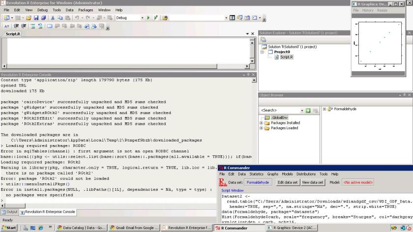
1) R Commander- R Commander was primarily created by Professor John Fox of McMaster University to cover the content of a basic statistics course. However it is extensible and many other packages can be added in menu form to it- in the form R Commander Plugins. Quite noticeably it is one of the most widely used R GUI and it also has a script window so you can write R code in combination with the menus.
As you point and click a particular menu item, the corresponding R code is automatically generated in the log window and executed.

It can be found on CRAN at http://cran.r-project.org/web/packages/Rcmdr/index.html


Advantages of Using  R Commander-
1) Useful for beginner in R language to do basic graphs and analysis and building models.
2) Has script window, output window and log window (called messages) in same screen which helps user as code is auto-generated on clicking on menus, and can be customized easily. For example in changing labels and options in Graphs.  Graphical output is shown in seperate window from output window.
3) Extensible for other R packages like qcc (for quality control), Teaching Demos (for training), survival analysis and Design of Experiments (DoE)
4) Easy to understand interface even for first time user.
5) Menu items which are not relevant are automatically greyed out- if there are only two variables, and you try to build a 3D scatterplot graph, that menu would simply not be available and is greyed out.

Comparative Disadvantages of using R Commander-
1) It is basically aimed at a statistical audience( originally students in statistics) and thus the terms as well as menus are accordingly labeled. Hence it is more of a statistical GUI rather than an analytics GUI.
2) Has limited ability to evaluate models from a business analysts perspective (ROC curve is not given as an option) even though it has extensive statistical tests for model evaluation in model sub menu. Indeed creating a Model is treated as a subsection of statistics rather than a separate menu item.
3) It is not suited for projects that do not involve advanced statistical testing and for users not proficient in statistics (particularly hypothesis testing), and for data miners.

Menu items in the R Commander window:
File Menu – For loading script files and saving Script files, Output and Workspace
It is also needed for changing the present working directory and for exiting R.
Edit Menu – For editing scripts and code in the script window.
Data Menu – For creating new dataset, inputting or importing data and manipulating data through variables. Data Import can be from text,comma separated values,clipboard, datasets from SPSS, Stata,Minitab, Excel ,dbase,  Access files or from url.
Data manipulation included deleting rows of data as well as manipulating variables.
Also this menu has the option for merging two datasets by row or columns.
Statistics Menu-This menu has options for descriptive statistics, hypothesis tests, factor analysis and clustering and also for creating models. Note there is a separate menu for evaluating the model so created.
Graphs Menu-It has options for creating various kinds of graphs including box-plot, histogram, line, pie charts and x-y plots.
The first option is color palette- it can be used for customizing the colors. It is recommended you adjust colors based on your need for publication or presentation.
A notable option is 3 D graphs for evaluating 3 variables at a time- this is really good and impressive feature and exposes the user to advanced graphs in R all at few clicks. You may want to dazzle a presentation using this graph.
Also consider scatterplot matrix graphs for graphical display of variables.
Graphical display of R surpasses any other statistical software in appeal as well as ease of creation- using GUI to create graphs can further help the user to get the most of data insights using R at a very minimum effort.
Models Menu-This is somewhat of a labeling peculiarity of R Commander as this menu is only for evaluating models which have been created using the statistics menu-model sub menu.
It includes options for graphical interpretation of model results,residuals,leverage and confidence intervals and adding back residuals to the data set.
Distributions Menu- is for cumulative probabilities, probability density, graphs of distributions, quantiles and features for standard distributions and can be used in lieu of standard statistical tables for the distributions. It has 13 standard statistical continuous distributions and 5 discrete distributions.
Tools Menu- allows you to load other packages and also load R Commander plugins (which are then added to the Interface Menu after the R Commander GUI is restarted). It also contains options sub menu for fine tuning (like opting to send output to R Menu)
Help Menu- Standard documentation and help menu. Essential reading is the short 25 page manual in it called Getting “Started With the R Commander”.

R Commander Plugins- There are twenty extensions to R Commander that greatly enhance it’s appeal -these include basic time series forecasting, survival analysis, qcc and more.

see a complete list at

  1. DoE – http://cran.r-project.org/web/packages/RcmdrPlugin.DoE/RcmdrPlugin.DoE.pdf
  2. doex
  3. EHESampling
  4. epack- http://cran.r-project.org/web/packages/RcmdrPlugin.epack/RcmdrPlugin.epack.pdf
  5. Export- http://cran.r-project.org/web/packages/RcmdrPlugin.Export/RcmdrPlugin.Export.pdf
  6. FactoMineR
  7. HH
  8. IPSUR
  9. MAc- http://cran.r-project.org/web/packages/RcmdrPlugin.MAc/RcmdrPlugin.MAc.pdf
  10. MAd
  11. orloca
  12. PT
  13. qcc- http://cran.r-project.org/web/packages/RcmdrPlugin.qcc/RcmdrPlugin.qcc.pdf and http://cran.r-project.org/web/packages/qcc/qcc.pdf
  14. qual
  15. SensoMineR
  16. SLC
  17. sos
  18. survival-http://cran.r-project.org/web/packages/RcmdrPlugin.survival/RcmdrPlugin.survival.pdf
  19. SurvivalT
  20. Teaching Demos

Note the naming convention for above e plugins is always with a Prefix of “RCmdrPlugin.” followed by the names above
Also on loading a Plugin, it must be already installed locally to be visible in R Commander’s list of load-plugin, and R Commander loads the e-plugin after restarting.Hence it is advisable to load all R Commander plugins in the beginning of the analysis session.

However the notable E Plugins are
1) DoE for Design of Experiments-
Full factorial designs, orthogonal main effects designs, regular and non-regular 2-level fractional
factorial designs, central composite and Box-Behnken designs, latin hypercube samples, and simple D-optimal designs can currently be generated from the GUI. Extensions to cover further latin hypercube designs as well as more advanced D-optimal designs (with blocking) are planned for the future.
2) Survival- This package provides an R Commander plug-in for the survival package, with dialogs for Cox models, parametric survival regression models, estimation of survival curves, and testing for differences in survival curves, along with data-management facilities and a variety of tests, diagnostics and graphs.
3) qcc -GUI for  Shewhart quality control charts for continuous, attribute and count data. Cusum and EWMA charts. Operating characteristic curves. Process capability analysis. Pareto chart and cause-and-effect chart. Multivariate control charts
4) epack- an Rcmdr “plug-in” based on the time series functions. Depends also on packages like , tseries, abind,MASS,xts,forecast. It covers Log-Exceptions garch
and following Models -Arima, garch, HoltWinters
5)Export- The package helps users to graphically export Rcmdr output to LaTeX or HTML code,
via xtable() or Hmisc::latex(). The plug-in was originally intended to facilitate exporting Rcmdr
output to formats other than ASCII text and to provide R novices with an easy-to-use,
easy-to-access reference on exporting R objects to formats suited for printed output. The
package documentation contains several pointers on creating reports, either by using
conventional word processors or LaTeX/LyX.
6) MAc- This is an R-Commander plug-in for the MAc package (Meta-Analysis with
Correlations). This package enables the user to conduct a meta-analysis in a menu-driven,
graphical user interface environment (e.g., SPSS), while having the full statistical capabilities of
R and the MAc package. The MAc package itself contains a variety of useful functions for
conducting a research synthesis with correlational data. One of the unique features of the MAc
package is in its integration of user-friendly functions to complete the majority of statistical steps
involved in a meta-analysis with correlations.
You can read more on R Commander Plugins at http://wp.me/p9q8Y-1Is
—————————————————————————————————————————-
Rattle- R Analytical Tool To Learn Easily (download from http://rattle.togaware.com/)
Rattle is more advanced user Interface than R Commander though not as popular in academia. It has been designed explicitly for data mining and it also has a commercial version for sale by Togaware. Rattle has a Tab and radio button/check box rather than Menu- drop down approach towards the graphical design. Also the Execute button needs to be clicked after checking certain options, just the same as submit button is clicked after writing code. This is different from clicking on a drop down menu.

Advantages of Using Rattle
1) Useful for beginner in R language to do building models,cluster and data mining.
2) Has separate tabs for data entry,summary, visualization,model building,clustering, association and evaluation. The design is intuitive and easy to understand even for non statistical background as the help is conveniently explained as each tab, button is clicked. Also the tabs are placed in a very sequential and logical order.
3) Uses a lot of other R packages to build a complete analytical platform. Very good for correlation graph,clustering as well decision trees.
4) Easy to understand interface even for first time user.
5) Log  for R code is auto generated and time stamp is placed.
6) Complete solution for model building from partitioning datasets randomly for testing,validation to building model, evaluating lift and ROC curve, and exporting PMML output of model for scoring.
7) Has a well documented online help as well as in-software documentation. The help helps explain terms even to non statistical users and is highly useful for business users.

Example Documentation for Hypothesis Testing in Test Tab in Rattle is ”
Distribution of the Data
* Kolomogorov-Smirnov     Non-parametric Are the distributions the same?
* Wilcoxon Signed Rank    Non-parametric Do paired samples have the same distribution?
Location of the Average
* T-test               Parametric     Are the means the same?
* Wilcoxon Rank-Sum    Non-parametric Are the medians the same?
Variation in the Data
* F-test Parametric Are the variances the same?
Correlation
* Correlation    Pearsons Are the values from the paired samples correlated?”

Comparative Disadvantages of using Rattle-
1) It is basically aimed at a data miner.  Hence it is more of a data mining GUI rather than an analytics GUI.
2) Has limited ability to create different types of graphs from a business analysts perspective Numeric variables can be made into Box-Plot, Histogram, Cumulative as well Benford Graphs. While interactivity using GGobi and Lattiticist is involved- the number of graphical options is still lesser than other GUI.
3) It is not suited for projects that involve multiple graphical analysis and which do not have model building or data mining.For example Data Plot is given in clustering tab but not in general Explore tab.
4) Despite the fact that it is meant for data miners, no support to biglm packages, as well as parallel programming is enabled in GUI for bigger datasets, though these can be done by R command line in conjunction with the Rattle GUI. Data m7ining is typically done on bigger datsets.
5) May have some problems installing it as it is dependent on GTK and has a lot of packages as dependencies.

Top Row-
This has the Execute Button (shown as two gears) and which has keyboard shortcut F2. It is used to execute the options in Tabs-and is equivalent of submit code button.
Other buttons include new Projects,Save  and Load projects which are files with extension to .rattle an which store all related information from Rattle.
It also has a button for exporting information in the current Tab as an open office document, and buttons for interrupting current process as well as exiting Rattle.

Data Tab-
It has the following options.
●        Data Type- These are radio buttons between Spreadsheet (and Comma Separated Values), ARFF files (Weka), ODBC (for Database Connections),Library (for Datasets from Packages),R Dataset or R datafile, Corpus (for Text Mining) and Script for generating the data by code.
●        The second row-in Data Tab in Rattle is Detail on Data Type- and its apperance shifts as per the radio button selection of data type in previous step. For Spreadsheet, it will show Path of File, Delimiters, Header Row while for ODBC it will show DSN, Tables, Rows and for Library it will show you a dropdown of all datasets in all R packages installed locally.
●        The third row is a Partition field for splitting dataset in training,testing,validation and it shows ratio. It also specifies a Random seed which can be customized for random partitions which can be replicated. This is very useful as model building requires model to be built and tested on random sub sets of full dataset.
●        The fourth row is used to specify the variable type of inputted data. The variable types are
○        Input: Used for modeling as independent variables
○        Target: Output for modeling or the dependent variable. Target is a categoric variable for classification, numeric for regression and for survival analysis both Time and Status need to be defined
○        Risk: A variable used in the Risk Chart
○        Ident: An identifier for unique observations in the data set like AccountId or Customer Id
○        Ignore: Variables that are to be ignored.
●        In addition the weight calculator can be used to perform mathematical operations on certain variables and identify certain variables as more important than others.

Explore Tab-
Summary Sub-Tab has Summary for brief summary of variables, Describe for detailed summary and Kurtosis and Skewness for comparing them across numeric variables.
Distributions Sub-Tab allows plotting of histograms, box plots, and cumulative plots for numeric variables and for categorical variables Bar Plot and Dot Plot.
It also has Benford Plot for Benford’s Law on probability of distribution of digits.
Correlation Sub-Tab– This displays corelation between variables as a table and also as a very nice plot.
Principal Components Sub-Tab– This is for use with Principal Components Analysis including the SVD (singular value decomposition) and Eigen methods.
Interactive Sub-Tab- Allows interactive data exploration using GGobi and Lattice software. It is a powerful visual tool.

Test Tab-This has options for hypothesis testing of data for two sample tests.
Transform Tab-This has options for rescaling data, missing values treatment, and deleting invalid or missing values.
Cluster Tab-It gives an option to KMeans, Hierarchical and Bi-Cluster clustering methods with automated graphs,plots (including dendogram, discriminant plot and data plot) and cluster results available. It is highly recommended for clustering projects especially for people who are proficient in clustering but not in R.

Associate Tab-It helps in building association rules between categorical variables, which are in the form of “if then”statements. Example. If day is Thursday, and someone buys Milk, there is 80% chance they will buy Diapers. These probabilities are generated from observed frequencies.

Model Tab-The Model tab makes Rattle one of the most advanced data mining tools, as it incorporates decision trees(including boosted models and forest method), linear and logistic regression, SVM,neural net,survival models.
Evaluate Tab-It as functionality for evaluating models including lift,ROC,confusion matrix,cost curve,risk chart,precision, specificity, sensitivity as well as scoring datasets with built model or models. Example – A ROC curve generated by Rattle for Survived Passengers in Titanic (as function of age,class,sex) This shows comparison of various models built.

Log Tab- R Code is automatically generated by Rattle as the respective operation is executed. Also timestamp is done so it helps in reviewing error as well as evaluating speed for code optimization.
—————————————————————————————————————————-
JGR- Deducer- (see http://www.deducer.org/pmwiki/pmwiki.php?n=Main.DeducerManual
JGR is a Java Based GUI. Deducer is recommended for use with JGR.
Deducer has basically been made to implement GGPLOT in a GUI- an advanced graphics package based on Grammer of Graphics and was part of Google Summer of Code project.

It first asks you to either open existing dataset or load a new dataset with just two icons. It has two initial views in Data Viewer- a Data view and Variable view which is quite similar to Base SPSS. The other Deducer options are loaded within the JGR console.

Advantages of Using  Deducer
1.      It has an option for factor as well as reliability analysis which is missing in other graphical user interfaces like R Commander and Rattle.
2.      The plot builder option gives very good graphics -perhaps the best in other GUIs. This includes a color by option which allows you to shade the colors based on variable value. An addition innovation is the form of templates which enables even a user not familiar with data visualization to choose among various graphs and click and drag them to plot builder area.
3.      You can set the Java Gui for R (JGR) menu to automatically load some packages by default using an easy checkbox list.
4.      Even though Deducer is a very young package, it offers a way for building other R GUIs using Java Widgets.
5.      Overall feel is of SPSS (Base GUI) to it’s drop down menu, and selecting variables in the sub menu dialogue by clicking to transfer to other side.SPSS users should be more comfortable at using this.
6.      A surprising thing is it rearranges the help documentation of all R in a very presentable and organized manner
7.      Very convenient to move between two or more datasets using dropdown.
8.      The most convenient GUI for merging two datasets using common variable.

Dis Advantages of Using  Deducer
1.      Not able to save plots as images (only options are .pdf and .eps), you can however copy as image.
2.      Basically a data viualization GUI – it does offer support for regression, descriptive statistics in the menu item Extras- however the menu suggests it is a work in progress.
3.      Website for help is outdated, and help documentation specific to Deducer lacks detail.


Components of Deducer-
Data Menu-Gives options for data manipulation including recoding variables,transform variables (binning, mathematical operation), sort dataset,  transpose dataset ,merge two datasets.
Analysis Menu-Gives options for frequency tables, descriptive statistics,cross tabs, one sample tests (with plots) ,two sample tests (with plots),k sample tests, correlation,linear and logistic models,generalized linear models.
Plot Builder Menu- This allows plots of various kinds to be made in an interactive manner.

Correlation using Deducer.

————————————————————————————————————————–
Red-R – A dataflow user interface for R (see http://red-r.org/

Red R uses dataflow concepts as a user interface rather than menus and tabs. Thus it is more similar to Enterprise Miner or Rapid Miner in design. For repeatable analysis dataflow programming is preferred by some analysts. Red-R is written in Python.


Advantages of using Red-R
1) Dataflow style makes it very convenient to use. It is the only dataflow GUI for R.
2) You can save the data as well as analysis in the same file.
3) User Interface makes it easy to read R code generated, and commit code.
4) For repeatable analysis-like reports or creating models it is very useful as you can replace just one widget and other widget/operations remain the same.
5) Very easy to zoom into data points by double clicking on graphs. Also to change colors and other options in graphs.
6) One minor feature- It asks you to set CRAN location just once and stores it even for next session.
7) Automated bug report submission.

Disadvantages of using Red-R
1) Current version is 1.8 and it needs a lot of improvement for building more modeling types as well as debugging errors.
2) Limited features presently.
———————————————————————————————————————-
RKWard (see http://rkward.sourceforge.net/)

It is primarily a KDE GUI for R, so it can be used on Ubuntu Linux. The windows version is available but has some bugs.

Advantages of using RKWard
1) It is the only R GUI for time series at present.
In addition it seems like the only R GUI explicitly for Item Response Theory (which includes credit response models,logistic models) and plots contains Pareto Charts.
2) It offers a lot of detail in analysis especially in plots(13 types of plots), analysis and  distribution analysis ( 8 Tests of normality,14 continuous and 6 discrete distributions). This detail makes it more suitable for advanced statisticians rather than business analytics users.
3) Output can be easily copied to Office documents.

Disadvantages of using RKWard
1) It does not have stable Windows GUI. Since a graphical user interface is aimed at making interaction easier for users- this is major disadvantage.
2) It has a lot of dependencies so may have some issues in installing.
3) The design categorization of analysis,plots and distributions seems a bit unbalanced considering other tabs are File, Edit, View, Workspace,Run,Settings, Windows,Help.
Some of the other tabs can be collapsed, while the three main tabs of analysis,plots,distributions can be better categorized (especially into modeling and non-modeling analysis).
4) Not many options for data manipulation (like subset or transpose) by the GUI.
5) Lack of detail in documentation as it is still on version 0.5.3 only.

Components-
Analysis, Plots and Distributions are the main components and they are very very extensive, covering perhaps the biggest range of plots,analysis or distribution analysis that can be done.
Thus RKWard is best combined with some other GUI, when doing advanced statistical analysis.


GNU General Public License
Image via Wikipedia

GrapherR

GrapheR is a Graphical User Interface created for simple graphs.

Depends: R (>= 2.10.0), tcltk, mgcv
Description: GrapheR is a multiplatform user interface for drawing highly customizable graphs in R. It aims to be a valuable help to quickly draw publishable graphs without any knowledge of R commands. Six kinds of graphs are available: histogram, box-and-whisker plot, bar plot, pie chart, curve and scatter plot.
License: GPL-2
LazyLoad: yes
Packaged: 2011-01-24 17:47:17 UTC; Maxime
Repository: CRAN
Date/Publication: 2011-01-24 18:41:47

More information about GrapheR at CRAN
Path: /cran/newpermanent link

Advantages of using GrapheR

  • It is bi-lingual (English and French) and can import in text and csv files
  • The intention is for even non users of R, to make the simple types of Graphs.
  • The user interface is quite cleanly designed. It is thus aimed as a data visualization GUI, but for a more basic level than Deducer.
  • Easy to rename axis ,graph titles as well use sliders for changing line thickness and color

Disadvantages of using GrapheR

  • Lack of documentation or help. Especially tips on mouseover of some options should be done.
  • Some of the terms like absicca or ordinate axis may not be easily understood by a business user.
  • Default values of color are quite plain (black font on white background).
  • Can flood terminal with lots of repetitive warnings (although use of warnings() function limits it to top 50)
  • Some of axis names can be auto suggested based on which variable s being chosen for that axis.
  • Package name GrapheR refers to a graphical calculator in Mac OS – this can hinder search engine results

Using GrapheR

  • Data Input -Data Input can be customized for CSV and Text files.
  • GrapheR gives information on loaded variables (numeric versus Factors)
  • It asks you to choose the type of Graph 
  • It then asks for usual Graph Inputs (see below). Note colors can be customized (partial window). Also number of graphs per Window can be easily customized 
  • Graph is ready for publication


Related Articles


Summary of R GUIs


Using R from other software- Please note that interfaces to R exist from other software as well. These include software from SAS Institute, IBM SPSS, Rapid Miner,Knime  and Oracle.

A brief list is shown below-

1) SAS/IML Interface to R- You can read about the SAS Institute’s SAS/ IML Studio interface to R at http://www.sas.com/technologies/analytics/statistics/iml/index.html
2) Rapid  Miner Extension to R-You can view integration with Rapid Miner’s extension to R here at http://www.youtube.com/watch?v=utKJzXc1Cow
3) IBM SPSS plugin for R-SPSS software has R integration in the form of a plugin. This was one of the earliest third party software offering interaction with R and you can read more at http://www.spss.com/software/statistics/developer/
4) Knime- Konstanz Information Miner also has R integration. You can view this on
http://www.knime.org/downloads/extensions
5) Oracle Data Miner- Oracle has a data mining offering to it’s very popular database software which is integrated with the R language. The R Interface to Oracle Data Mining ( R-ODM) allows R users to access the power of Oracle Data Mining’s in-database functions using the familiar R syntax. http://www.oracle.com/technetwork/database/options/odm/odm-r-integration-089013.html
6) JMP- JMP version 9 is the latest to offer interface to R.  You can read example scripts here at http://blogs.sas.com/jmp/index.php?/archives/298-JMP-Into-R!.html

R Excel- Using R from Microsoft Excel

Microsoft Excel is the most widely used spreadsheet program for data manipulation, entry and graphics. Yet as dataset sizes have increased, Excel’s statistical capabilities have lagged though it’s design has moved ahead in various product versions.

R Excel basically works at adding a .xla plugin to
Excel just like other Plugins. It does so by connecting to R through R packages.

Basically it offers the functionality of R
functions and capabilities to the most widely distributed spreadsheet program. All data summaries, reports and analysis end up in a spreadsheet-

R Excel enables R to be very useful for people not
knowing R. In addition it adds (by option) the menus of R Commander as menus in Excel spreadsheet.


Advantages-
Enables R and Excel to communicate thus tieing an advanced statistical tool to the most widely used business analytics tool.

Disadvantages-
No major disadvatage at all to a business user. For a data statistical user, Microsoft Excel is limited to 100,000 rows, so R data needs to be summarized or reduced.

Graphical capabilities of R are very useful, but to a new user, interactive graphics in Excel may be easier than say using Ggplot ot Ggobi.
You can read more on this at http://rcom.univie.ac.at/ or  the complete Springer Book http://www.springer.com/statistics/computanional+statistics/book/978-1-4419-0051-7

The combination of cloud computing and internet offers a new kind of interaction possible for scientists as well analysts.

Here is a way to use R on an Amazon EC2 machine, thus renting by hour hardware and computing resources which are scaleable to massive levels , whereas the software is free.

Here is how you can connect to Amazon EC2 and run R.
Running R for Cloud Computing.
1) Logging onto Amazon Console http://aws.amazon.com/ec2/
Note you need your Amazon Id (even the same id which you use for buying books).Note we are into Amazon EC2 as shown by the upper tab. Click upper tab to get into the Amazon EC2
2) Choosing the right AMI-On the left margin, you can click AMI -Images. Now you can search for the image-I chose Ubuntu images (linux images are cheaper) and latest Ubuntu Lucid  in the search .You can choose whether you want 32 bit or 64 bit image. 64 bit images will lead to  faster processing of data.Click on launch instance in the upper tab ( near the search feature). A pop up comes up, which shows the 5 step process to launch your computing.
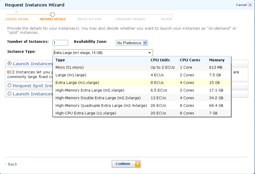
3) Choose the right compute instance- – there are various compute instances and they all are at different multiples of prices or compute units. They differ in terms of RAM memory and number of processors.After choosing the compute instance of your choice (extra large is highlighted)- click on continue-
4) Instance Details-Do not  choose cloudburst monitoring if you are on a budget as it has a extra charge. For critical production it would be advisable to choose cloudburst monitoring once you have become comfortable with handling cloud computing..
5) Add Tag Details- If you are running a lot of instances you need to create your own tags to help you manage them. It is advisable if you are going to run many instances.
6) Create a key pair- A key pair is an added layer of encryption. Click on create new pair and name it (note the name will be handy in coming steps)
7) After clicking and downloading the key pair- you come into security groups. Security groups is just a set of instructions to help keep your data transfer secure. You want to enable access to your cloud instance to certain IP addresses (if you are going to connect from fixed IP address and to certain ports in your computer. It is necessary in security group to enable  SSH using Port 22.
Last step- Review Details and Click Launch
8) On the Left margin click on instances ( you were in Images.>AMI earlier)
It will take some 3-5 minutes to launch an instance. You can see status as pending till then.
9) Pending instance as shown by yellow light-
10) Once the instance is running -it is shown by a green light.
Click on the check box, and on upper tab go to instance actions. Click on connect-
You see a popup with instructions like these-
· Open the SSH client of your choice (e.g., PuTTY, terminal).
·  Locate your private key, nameofkeypair.pem
·  Use chmod to make sure your key file isn’t publicly viewable, ssh won’t work otherwise:
chmod 400 decisionstats.pem
·  Connect to your instance using instance’s public DNS [ec2-75-101-182-203.compute-1.amazonaws.com].
Example
Enter the following command line:
ssh -i decisionstats2.pem root@ec2-75-101-182-203.compute-1.amazonaws.com

Note- If you are using Ubuntu Linux on your desktop/laptop you will need to change the above line to ubuntu@… from root@..

ssh -i yourkeypairname.pem -X ubuntu@ec2-75-101-182-203.compute-1.amazonaws.com

(Note X11 package should be installed for Linux users- Windows Users will use Remote Desktop)

12) Install R Commander on the remote machine (which is running Ubuntu Linux) using the command

sudo apt-get install r-cran-rcmdr


Using Code Editors in R

Using Enhanced Code Editors


Advantages of using enhanced code editors

1) Readability- Features like syntax coloring helps make the code more readable for documentation as well as debugging and improvement. Example functions may be colored in blue, input parameters in green, and simple default code syntax in black. Especially for lengthy programs or tweaking auto generated code by GUI, this readability comes in handy.

2) Automatic syntax error checking- Enhanced editors can prompt you if certain errors in syntax (like brackets not closed, commas misplaced)- and errors may be highlighted in color (red mostly). This helps a lot in correcting code especially if you are either new to R programming or your main focus is business insights and not just coding. Syntax debugging is thus simplified.

3) Speed of writing code- Most programmers report an increase in writing code speed when using an enhanced editor.

4) Point Breaks- You can insert breaks at certain parts of code to run some lines of code together, or debug a program. This is a big help given that default code editor makes it very cumbersome and you have to copy and paste lines of code again and again to run selectively. On an enhanced editor you can submit lines as well as paragraphs of code.

5) Auto-Completion- Auto completion enables or suggests options you to complete the syntax even when you have typed part of the function name.

Some commonly used code editors are –
Notepad++ -It supports R and also has a plugin called NPP to R.
It can be used  for a wide variety of other languages as well, and has all the features mentioned above.

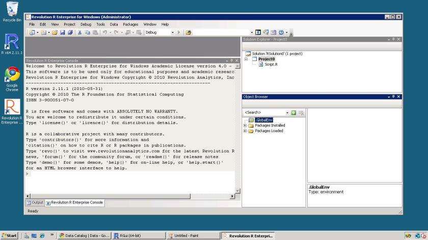
Revolution R Productivity Environment (RPE)-While Revolution R has announced a new GUI to be launched in 2011- the existing enhancements to their software include a code editor called RPE.

Syntax color highlighting is already included. Code Snippets work in a fairly simply way.
Right click-
Click on Insert Code Snippet.

You can get a drop down of tasks to do- (like Analysis)
Selecting Analysis we get another list of sub-tasks (like Clustering).
Once you click on Clustering you get various options.
Like clicking clara will auto insert the code for clara clustering.

Now even if you are averse to using a GUI /or GUI creators don’t have your particular analysis you can basically type in code at an extremely fast pace.
It is useful to even experienced people who do not have to type in the entire code, but it is a boon to beginners as the parameters in function inserted by code snippet are automatically selected in multiple colors. And it can help you modify the auto generated code by your R GUI at a much faster pace.

TinnR -The most popular and a very easy to use code editor. It is available at http://www.sciviews.org/Tinn-R/
It’s disadvantage is it supports Windows operating system only.
Recommended as the beginner’s chose fore code editor.

Eclipse with R plugin http://www.walware.de/goto/statet This is recommended especially to people working with Eclipse and on Unix systems. It enables you to do most of the productivity enhancement featured in other text editors including submitting code the R session.

Gvim (http://www.vim.org/) along Vim-R-plugin2
(http://www.vim.org/scripts/script.php?script_id=2628) should be
cited. The Vim-R-plugin developer recently added windows support to a
lean cross-platform package that works well. It can be suited as a niche text editor to people who like less features in the software. It is not as good as Eclipse or Notepad++ but is probably the simplest to use.

R on Windows HPC Server

From HPC Wire, the newsletter/site for all HPC news-

Source- Link

PALO ALTO, Calif., Sept. 20 — Revolution Analytics, the leading commercial provider of software and support for the popular open source R statistics language, today announced it will deliver Revolution R Enterprise for Microsoft Windows HPC Server 2008 R2, released today, enabling users to analyze very large data sets in high-performance computing environments.

R is a powerful open source statistics language and the modern system for predictive analytics. Revolution Analytics recently introduced RevoScaleR, new “Big Data” analysis capabilities, to its R distribution, Revolution R Enterprise. RevoScaleR solves the performance and capacity limitations of the R language by with parallelized algorithms that stream data across multiple cores on a laptop, workstation or server. Users can now process, visualize and model terabyte-class data sets at top speeds — without the need for specialized hardware.

“Revolution Analytics is pleased to support Microsoft’s Technical Computing initiative, whose efforts will benefit scientists, engineers and data analysts,” said David Champagne, CTO at Revolution. “We believe the engineering we have done for Revolution R Enterprise, in particular our work on big-data statistics and multicore computing, along with Microsoft’s HPC platform for technical computing, makes an ideal combination for high-performance large scale statistical computing.”

“Processing and analyzing this ‘big data’ is essential to better prediction and decision making,” said Bill Hamilton, director of technical computing at Microsoft Corp. “Revolution R Enterprise for Windows HPC Server 2008 R2 gives customers an extremely powerful tool that handles analysis of very large data and high workloads.”

To learn more about Revolution R Enterprise and its Big Data capabilities, download thewhite paper. Revolution Analytics also has an on-demand webcast, “High-performance analytics with Revolution R and Windows HPC Server,” available online.

AND from Microsoft’s website

http://www.microsoft.com/hpc/en/us/solutions/hpc-for-life-sciences.aspx

REvolution R Enterprise »

REvolution Computing

REvolution R Enterprise is designed for both novice and experienced R users looking for a production-grade R distribution to perform mission critical predictive analytics tasks right from the desktop and scale across multiprocessor environments. Featuring RPE™ REvolution’s R Productivity Environment for Windows.

Of course R Enterprise is available on Linux but on Red Hat Enterprise Linux- it would be nice to see Amazom Machine Images as well as Ubuntu versions as well.

An Amazon Machine Image (AMI) is a special type of virtual appliance which is used to instantiate (create) a virtual machine within the Amazon Elastic Compute Cloud. It serves as the basic unit of deployment for services delivered using EC2.[1]

Like all virtual appliances, the main component of an AMI is a read-only filesystem image which includes an operating system (e.g., Linux, UNIX, or Windows) and any additional software required to deliver a service or a portion of it.[2]

The AMI filesystem is compressed, encrypted, signed, split into a series of 10MB chunks and uploaded into Amazon S3 for storage. An XML manifest file stores information about the AMI, including name, version, architecture, default kernel id, decryption key and digests for all of the filesystem chunks.

An AMI does not include a kernel image, only a pointer to the default kernel id, which can be chosen from an approved list of safe kernels maintained by Amazon and its partners (e.g., RedHat, Canonical, Microsoft). Users may choose kernels other than the default when booting an AMI.[3]

[edit]Types of images

  • Public: an AMI image that can be used by any one.
  • Paid: a for-pay AMI image that is registered with Amazon DevPay and can be used by any one who subscribes for it. DevPay allows developers to mark-up Amazon’s usage fees and optionally add monthly subscription fees.

SAS/Blades/Servers/ GPU Benchmarks

Just checked out cool new series from NVidia servers.

Now though SAS Inc/ Jim Goodnight thinks HP Blade Servers are the cool thing- the GPU takes hardware high performance computing to another level. It would be interesting to see GPU based cloud computers as well – say for the on Demand SAS (free for academics and students) but which has had some complaints of being slow.

See this for SAS and Blade Servers-

http://www.sas.com/success/ncsu_analytics.html

To give users hands-on experience, the program is underpinned by a virtual computing lab (VCL), a remote access service that allows users to reserve a computer configured with a desired set of applications and operating system and then access that computer over the Internet. The lab is powered by an IBM BladeCenter infrastructure, which includes more than 500 blade servers, distributed between two locations. The assignment of the blade servers can be changed to meet shifts in the balance of demand among the various groups of users. Laura Ladrie, MSA Classroom Coordinator and Technical Support Specialist, says, “The virtual computing lab chose IBM hardware because of its quality, reliability and performance. IBM hardware is also energy efficient and lends itself well to high performance/low overhead computing.

Thats interesting since IBM now competes (as owner of SPSS) and also cooperates with SAS Institute

And

http://www.theaustralian.com.au/australian-it/the-world-according-to-jim-goodnight-blade-switch-slashes-job-times/story-e6frgakx-1225888236107

You’re effectively turbo-charging through deployment of many processors within the blade servers?

Yes. We’ve got machines with 192 blades on them. One of them has 202 or 203 blades. We’re using Hewlett-Packard blades with 12 CP cores on each, so it’s a total 2300 CPU cores doing the computation.

Our idea was to give every one of those cores a little piece of work to do, and we came up with a solution. It involved a very small change to the algorithm we were using, and it’s just incredible how fast we can do things now.

I don’t think of it as a grid, I think of it as essentially one computer. Most people will take a blade and make a grid out of it, where everything’s a separate computer running separate jobs.

We just look at it as one big machine that has memory and processors all over the place, so it’s a totally different concept.

GPU servers can be faster than CPU servers, though , Professor G.


Source-

http://www.nvidia.com/object/preconfigured_clusters.html

TESLA GPU COMPUTING SOLUTIONS FOR DATA CENTERS
Supercharge your cluster with the Tesla family of GPU computing solutions. Deploy 1U systems from NVIDIA or hybrid CPU-GPU servers from OEMs that integrate NVIDIA® Tesla™ GPU computing processors.

When compared to the latest quad-core CPU, Tesla 20-series GPU computing processors deliver equivalent performance at 1/20th the power consumption and 1/10th the cost. Each Tesla GPU features hundreds of parallel CUDA cores and is based on the revolutionary NVIDIA® CUDA™ parallel computing architecture with a rich set of developer tools (compilers, profilers, debuggers) for popular programming languages APIs like C, C++, Fortran, and driver APIs like OpenCL and DirectCompute.

NVIDIA’s partners provide turnkey easy-to-deploy Preconfigured Tesla GPU clusters that are customizable to your needs. For 3D cloud computing applications, our partners offer the Tesla RS clusters that are optimized for running RealityServer with iray.

Available Tesla Products for Data Centers:
– Tesla S2050
– Tesla M2050/M2070
– Tesla S1070
– Tesla M1060

Also I liked the hybrid GPU and CPU

And from a paper on comparing GPU and CPU using Benchmark tests on BLAS from a Debian- Dirk E’s excellent blog

http://dirk.eddelbuettel.com/blog/

Usage of accelerated BLAS libraries seems to shrouded in some mystery, judging from somewhat regularly recurring requests for help on lists such as r-sig-hpc(gmane version), the R list dedicated to High-Performance Computing. Yet it doesn’t have to be; installation can be really simple (on appropriate systems).

Another issue that I felt needed addressing was a comparison between the different alternatives available, quite possibly including GPU computing. So a few weeks ago I sat down and wrote a small package to run, collect, analyse and visualize some benchmarks. That package, called gcbd (more about the name below) is now onCRAN as of this morning. The package both facilitates the data collection for the paper it also contains (in the vignette form common among R packages) and provides code to analyse the data—which is also included as a SQLite database. All this is done in the Debian and Ubuntu context by transparently installing and removing suitable packages providing BLAS implementations: that we can fully automate data collection over several competing implementations via a single script (which is also included). Contributions of benchmark results is encouraged—that is the idea of the package.

And from his paper on the same-

Analysts are often eager to reap the maximum performance from their computing platforms.

A popular suggestion in recent years has been to consider optimised basic linear algebra subprograms (BLAS). Optimised BLAS libraries have been included with some (commercial) analysis platforms for a decade (Moler 2000), and have also been available for (at least some) Linux distributions for an equally long time (Maguire 1999). Setting BLAS up can be daunting: the R language and environment devotes a detailed discussion to the topic in its Installation and Administration manual (R Development Core Team 2010b, appendix A.3.1). Among the available BLAS implementations, several popular choices have emerged. Atlas (an acronym for Automatically Tuned Linear Algebra System) is popular as it has shown very good performance due to its automated and CPU-speci c tuning (Whaley and Dongarra 1999; Whaley and Petitet 2005). It is also licensed in such a way that it permits redistribution leading to fairly wide availability of Atlas.1 We deploy Atlas in both a single-threaded and a multi-threaded con guration. Another popular BLAS implementation is Goto BLAS which is named after its main developer, Kazushige Goto (Goto and Van De Geijn 2008). While `free to use’, its license does not permit redistribution putting the onus of con guration, compilation and installation on the end-user. Lastly, the Intel Math Kernel Library (MKL), a commercial product, also includes an optimised BLAS library. A recent addition to the tool chain of high-performance computing are graphical processing units (GPUs). Originally designed for optimised single-precision arithmetic to accelerate computing as performed by graphics cards, these devices are increasingly used in numerical analysis. Earlier criticism of insucient floating-point precision or severe performance penalties for double-precision calculation are being addressed by the newest models. Dependence on particular vendors remains a concern with NVidia’s CUDA toolkit (NVidia 2010) currently still the preferred development choice whereas the newer OpenCL standard (Khronos Group 2008) may become a more generic alternative that is independent of hardware vendors. Brodtkorb et al. (2010) provide an excellent recent survey. But what has been lacking is a comparison of the e ective performance of these alternatives. This paper works towards answering this question. By analysing performance across ve di erent BLAS implementations|as well as a GPU-based solution|we are able to provide a reasonably broad comparison.

Performance is measured as an end-user would experience it: we record computing times from launching commands in the interactive R environment (R Development Core Team 2010a) to their completion.

And

Basic Linear Algebra Subprograms (BLAS) provide an Application Programming Interface
(API) for linear algebra. For a given task such as, say, a multiplication of two conformant
matrices, an interface is described via a function declaration, in this case sgemm for single
precision and dgemm for double precision. The actual implementation becomes interchangeable
thanks to the API de nition and can be supplied by di erent approaches or algorithms. This
is one of the fundamental code design features we are using here to benchmark the di erence
in performance from di erent implementations.
A second key aspect is the di erence between static and shared linking. In static linking,
object code is taken from the underlying library and copied into the resulting executable.
This has several key implications. First, the executable becomes larger due to the copy of
the binary code. Second, it makes it marginally faster as the library code is present and
no additional look-up and subsequent redirection has to be performed. The actual amount
of this performance penalty is the subject of near-endless debate. We should also note that
this usually amounts to only a small load-time penalty combined with a function pointer
redirection|the actual computation e ort is unchanged as the actual object code is identi-
cal. Third, it makes the program more robust as fewer external dependencies are required.
However, this last point also has a downside: no changes in the underlying library will be
reected in the binary unless a new build is executed. Shared library builds, on the other
hand, result in smaller binaries that may run marginally slower|but which can make use of
di erent libraries without a rebuild.

Basic Linear Algebra Subprograms (BLAS) provide an Application Programming Interface(API) for linear algebra. For a given task such as, say, a multiplication of two conformantmatrices, an interface is described via a function declaration, in this case sgemm for singleprecision and dgemm for double precision. The actual implementation becomes interchangeablethanks to the API de nition and can be supplied by di erent approaches or algorithms. Thisis one of the fundamental code design features we are using here to benchmark the di erencein performance from di erent implementations.A second key aspect is the di erence between static and shared linking. In static linking,object code is taken from the underlying library and copied into the resulting executable.This has several key implications. First, the executable becomes larger due to the copy ofthe binary code. Second, it makes it marginally faster as the library code is present andno additional look-up and subsequent redirection has to be performed. The actual amountof this performance penalty is the subject of near-endless debate. We should also note thatthis usually amounts to only a small load-time penalty combined with a function pointerredirection|the actual computation e ort is unchanged as the actual object code is identi-cal. Third, it makes the program more robust as fewer external dependencies are required.However, this last point also has a downside: no changes in the underlying library will bereected in the binary unless a new build is executed. Shared library builds, on the otherhand, result in smaller binaries that may run marginally slower|but which can make use ofdi erent libraries without a rebuild.

And summing up,

reference BLAS to be dominated in all cases. Single-threaded Atlas BLAS improves on the reference BLAS but loses to multi-threaded BLAS. For multi-threaded BLAS we nd the Goto BLAS dominate the Intel MKL, with a single exception of the QR decomposition on the xeon-based system which may reveal an error. The development version of Atlas, when compiled in multi-threaded mode is competitive with both Goto BLAS and the MKL. GPU computing is found to be compelling only for very large matrix sizes. Our benchmarking framework in the gcbd package can be employed by others through the R packaging system which could lead to a wider set of benchmark results. These results could be helpful for next-generation systems which may need to make heuristic choices about when to compute on the CPU and when to compute on the GPU.

Source – DirkE’paper and blog http://dirk.eddelbuettel.com/papers/gcbd.pdf

Quite appropriately-,

Hardware solutions or atleast need to be a part of Revolution Analytic’s thinking as well. SPSS does not have any choice anymore though 😉

It would be interesting to see how the new SAS Cloud Computing/ Server Farm/ Time Sharing facility is benchmarking CPU and GPU for SAS analytics performance – if being done already it would be nice to see a SUGI paper on the same at http://sascommunity.org.

Multi threading needs to be taken care automatically by statistical software to optimize current local computing (including for New R)

Acceptable benchmarks for testing hardware as well as software need to be reinforced and published across vendors, academics  and companies.

What do you think?


The Cloud OS is finally here or is it?: Karmic Koala

Screenshot-34

see screenshot for cloud OS services in latest version of Ubuntu tobe launched in 5 days at http://www.ubuntu.com

( I am using the 9.10 latest beta since I figured 5 days earlier beta should be okay)

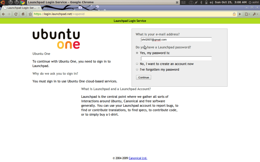
The Cloud OS properties are using browser and are called Ubuntu One

The browser used is Google Chrome.

Nice one, stanford dropouts. Really nice!

Note the line launchpad based services and uses secure id to ensure a connection as well as collect data for analysis as well

as real estate for possible advertisements.

Ball in Uncle Billy ‘s court now.

Note-The icon had some issues with opening more than one session parallely and showed edit preferences. So it could be a Google Joke as well

Easter Egg with an April variation. LOL

%d bloggers like this: