July 2017 – DECISION STATS

Finding out Environmental Variables in Windows

Use cmd to get the terminal

Then type SET to get the environmental variables

C:\Users\AJAY>SET

test and control split prior to modeling in SAS language #sasstats

https://github.com/decisionstats/sas-for-data-science/blob/master/split%20test%20and%20control.sas

Screenshot from 2017-07-12 16-20-59

data cars;

set sashelp.cars;

run;

data cars2;

set sashelp.cars;

where ranuni(12) <=.25;

run;

data cars2;

set sashelp.cars;

where ranuni(12) <=.25;

run;

NOTE: There were 114 observations read from the data set SASHELP.CARS.

WHERE RANUNI(12)<=0.25;

NOTE: The data set WORK.CARS2 has 114 observations and 15 variables.

data cars3 cars4;

set sashelp.cars;

if ranuni(12)<=.25 then output cars3;

else output cars4;

run;

data cars3 cars4;

set sashelp.cars;

if ranuni(12)<=.25 then output cars3;

else output cars4;

run;

NOTE: There were 428 observations read from the data set SASHELP.CARS.

NOTE: The data set WORK.CARS3 has 114 observations and 15 variables.

NOTE: The data set WORK.CARS4 has 314 observations and 15 variables.

PROC SURVEYSELECT DATA=cars OUT=test_cars METHOD=srs SAMPRATE=0.25;

RUN;

PROC SURVEYSELECT DATA=cars outall OUT=test_cars2 METHOD=srs SAMPRATE=0.25;

RUN;

PROC SURVEYSELECT DATA=cars OUT=test_cars METHOD=srs SAMPRATE=0.25;

RUN;

NOTE: The data set WORK.TEST_CARS has 107 observations and 15 variables.

NOTE: PROCEDURE SURVEYSELECT used (Total process time):

PROC SURVEYSELECT DATA=cars outall OUT=test_cars2 METHOD=srs SAMPRATE=0.25;

RUN;

NOTE: The data set WORK.TEST_CARS2 has 428 observations and 16 variables.

NOTE: PROCEDURE SURVEYSELECT used (Total process time):

proc print data=test_cars2 (obs=6);

var selected;

run;

proc freq data=test_cars2;

tables selected/norow nocol nocum nopercent;

run;

data test ;

set test_cars2;

where selected=0 ;

run;

data control ;

set test_cars2;

where selected=1 ;

run;

Output

Automated Machine Learning using Python TPot

Python Tpot offers automated machine learning.

From

Click to access olson_tpot_2016.pdf

Machine learning is commonly described as a field of study that gives computers the ability to learn without being explicitly programmed”(Simon, 2013). Despite this common claim, machine learning practitioners know that designing effective machine learning pipelines is often a tedious endeavour, and typically requires considerable experience with machine learning algorithms, expert knowledge of the problem domain, and brute force search to accomplish (Olson et al., 2016a). Thus, contrary to what machine learning enthusiasts would have us believe, machine learning still requires considerable explicit programming. In response to this challenge, several automated machine learning methods have been developed over the years (Hutter et al., 2015).

Over the past year, we have been developing a Tree-based Pipeline Optimization Tool (TPOT) that automatically designs and optimizes machine learning pipelines for a given problem domain (Olson et al., 2016b), without any need for human intervention. In short, TPOT optimizes machine learning pipelines using a version of genetic programming (GP)

http://rhiever.github.io/tpot/ and https://github.com/rhiever/tpot

TPOT is built on top of scikit-learn, so all of the code it generates should look familiar… if you’re familiar with scikit-learn, anyway.

and

Citation: Evaluation of a Tree-based Pipeline Optimization Tool for Automating Data Science

Randal S. Olson, Nathan Bartley, Ryan J. Urbanowicz, and Jason H. Moore (2016). Evaluation of a Tree-based Pipeline Optimization Tool for Automating Data Science. Proceedings of GECCO 2016, pages 485-492

Decision Trees in R simplified

library(rattle)

## Rattle: A free graphical interface for data mining with R.
## Version 4.1.0 Copyright (c) 2006-2015 Togaware Pty Ltd.
## Type 'rattle()' to shake, rattle, and roll your data.

library(party)

## Loading required package: grid

## Loading required package: mvtnorm

## Loading required package: modeltools

## Loading required package: stats4

## Loading required package: strucchange

## Loading required package: zoo

## 
## Attaching package: 'zoo'

## The following objects are masked from 'package:base':
## 
##     as.Date, as.Date.numeric

## Loading required package: sandwich

data(iris)
model=ctree(Species~.,data = iris)
plot(model)

table(predict(model),iris$Species)

##             
##              setosa versicolor virginica
##   setosa         50          0         0
##   versicolor      0         49         5
##   virginica       0          1        45

library(rpart)


model2=rpart(Species~.,data = iris)
fancyRpartPlot(model2)

library(randomForest)

## randomForest 4.6-12

## Type rfNews() to see new features/changes/bug fixes.

model3=randomForest(Species~.,data = iris)
table(predict(model3),iris$Species)

##             
##              setosa versicolor virginica
##   setosa         50          0         0
##   versicolor      0         47         4
##   virginica       0          3        46

K Means Clustering in Python

from https://github.com/decisionstats/pythonfordatascience/blob/master/2%2BClustering%2B-K%2BMeans.ipynb


import matplotlib.pyplot as plt
from sklearn import datasets
from sklearn.cluster import KMeans
import sklearn.metrics as sm
 
import pandas as pd
import numpy as np

In [2]:

wine=pd.read_csv("http://archive.ics.uci.edu/ml/machine-learning-databases/wine/wine.data",header=None)

In [3]:

wine.head()

Out[3]:

	0	1	2	3	4	5	6	7	8	9	10	11	12	13
0	1	14.23	1.71	2.43	15.6	127	2.80	3.06	0.28	2.29	5.64	1.04	3.92	1065
1	1	13.20	1.78	2.14	11.2	100	2.65	2.76	0.26	1.28	4.38	1.05	3.40	1050
2	1	13.16	2.36	2.67	18.6	101	2.80	3.24	0.30	2.81	5.68	1.03	3.17	1185
3	1	14.37	1.95	2.50	16.8	113	3.85	3.49	0.24	2.18	7.80	0.86	3.45	1480
4	1	13.24	2.59	2.87	21.0	118	2.80	2.69	0.39	1.82	4.32	1.04	2.93	735

In [4]:

wine.columns=['winetype','Alcohol','Malic acid','Ash','Alcalinity of ash','Magnesium','Total phenols','Flavanoids','Nonflavanoid phenols','Proanthocyanins','Color intensity','Hue','OD280/OD315 of diluted wines','Proline']

In [5]:

wine.head()

Out[5]:

	winetype	Alcohol	Malic acid	Ash	Alcalinity of ash	Magnesium	Total phenols	Flavanoids	Nonflavanoid phenols	Proanthocyanins	Color intensity	Hue	OD280/OD315 of diluted wines	Proline
0	1	14.23	1.71	2.43	15.6	127	2.80	3.06	0.28	2.29	5.64	1.04	3.92	1065
1	1	13.20	1.78	2.14	11.2	100	2.65	2.76	0.26	1.28	4.38	1.05	3.40	1050
2	1	13.16	2.36	2.67	18.6	101	2.80	3.24	0.30	2.81	5.68	1.03	3.17	1185
3	1	14.37	1.95	2.50	16.8	113	3.85	3.49	0.24	2.18	7.80	0.86	3.45	1480
4	1	13.24	2.59	2.87	21.0	118	2.80	2.69	0.39	1.82	4.32	1.04	2.93	735

In [6]:

wine.info()

<class 'pandas.core.frame.DataFrame'>
RangeIndex: 178 entries, 0 to 177
Data columns (total 14 columns):
winetype                        178 non-null int64
Alcohol                         178 non-null float64
Malic acid                      178 non-null float64
Ash                             178 non-null float64
Alcalinity of ash               178 non-null float64
Magnesium                       178 non-null int64
Total phenols                   178 non-null float64
Flavanoids                      178 non-null float64
Nonflavanoid phenols            178 non-null float64
Proanthocyanins                 178 non-null float64
Color intensity                 178 non-null float64
Hue                             178 non-null float64
OD280/OD315 of diluted wines    178 non-null float64
Proline                         178 non-null int64
dtypes: float64(11), int64(3)
memory usage: 19.5 KB

In [7]:

wine.describe()

Out[7]:

	winetype	Alcohol	Malic acid	Ash	Alcalinity of ash	Magnesium	Total phenols	Flavanoids	Nonflavanoid phenols	Proanthocyanins	Color intensity	Hue	OD280/OD315 of diluted wines	Proline
count	178.000000	178.000000	178.000000	178.000000	178.000000	178.000000	178.000000	178.000000	178.000000	178.000000	178.000000	178.000000	178.000000	178.000000
mean	1.938202	13.000618	2.336348	2.366517	19.494944	99.741573	2.295112	2.029270	0.361854	1.590899	5.058090	0.957449	2.611685	746.893258
std	0.775035	0.811827	1.117146	0.274344	3.339564	14.282484	0.625851	0.998859	0.124453	0.572359	2.318286	0.228572	0.709990	314.907474
min	1.000000	11.030000	0.740000	1.360000	10.600000	70.000000	0.980000	0.340000	0.130000	0.410000	1.280000	0.480000	1.270000	278.000000
25%	1.000000	12.362500	1.602500	2.210000	17.200000	88.000000	1.742500	1.205000	0.270000	1.250000	3.220000	0.782500	1.937500	500.500000
50%	2.000000	13.050000	1.865000	2.360000	19.500000	98.000000	2.355000	2.135000	0.340000	1.555000	4.690000	0.965000	2.780000	673.500000
75%	3.000000	13.677500	3.082500	2.557500	21.500000	107.000000	2.800000	2.875000	0.437500	1.950000	6.200000	1.120000	3.170000	985.000000
max	3.000000	14.830000	5.800000	3.230000	30.000000	162.000000	3.880000	5.080000	0.660000	3.580000	13.000000	1.710000	4.000000	1680.000000

In [8]:

pd.value_counts(wine['winetype'])

Out[8]:

2    71
1    59
3    48
Name: winetype, dtype: int64

In [9]:

x=wine.ix[:,1:14]
y=wine.ix[:,:1]

In [10]:

x.columns

Out[10]:

Index(['Alcohol', 'Malic acid', 'Ash', 'Alcalinity of ash', 'Magnesium',
       'Total phenols', 'Flavanoids', 'Nonflavanoid phenols',
       'Proanthocyanins', 'Color intensity', 'Hue',
       'OD280/OD315 of diluted wines', 'Proline'],
      dtype='object')

In [11]:

y.columns

Out[11]:

Index(['winetype'], dtype='object')

In [12]:

x.head()

Out[12]:

	Alcohol	Malic acid	Ash	Alcalinity of ash	Magnesium	Total phenols	Flavanoids	Nonflavanoid phenols	Proanthocyanins	Color intensity	Hue	OD280/OD315 of diluted wines	Proline
0	14.23	1.71	2.43	15.6	127	2.80	3.06	0.28	2.29	5.64	1.04	3.92	1065
1	13.20	1.78	2.14	11.2	100	2.65	2.76	0.26	1.28	4.38	1.05	3.40	1050
2	13.16	2.36	2.67	18.6	101	2.80	3.24	0.30	2.81	5.68	1.03	3.17	1185
3	14.37	1.95	2.50	16.8	113	3.85	3.49	0.24	2.18	7.80	0.86	3.45	1480
4	13.24	2.59	2.87	21.0	118	2.80	2.69	0.39	1.82	4.32	1.04	2.93	735

In [13]:

y.head()

Out[13]:

	winetype
0	1
1	1
2	1
3	1
4	1

In [14]:

# K Means Cluster
model = KMeans(n_clusters=3)
model.fit(x)

Out[14]:

KMeans(copy_x=True, init='k-means++', max_iter=300, n_clusters=3, n_init=10,
    n_jobs=1, precompute_distances='auto', random_state=None, tol=0.0001,
    verbose=0)

In [15]:

model.labels_

Out[15]:

array([1, 1, 1, 1, 2, 1, 1, 1, 1, 1, 1, 1, 1, 1, 1, 1, 1, 1, 1, 2, 2, 2, 1,
       1, 2, 2, 1, 1, 2, 1, 1, 1, 1, 1, 1, 2, 2, 1, 1, 2, 2, 1, 1, 2, 2, 1,
       1, 1, 1, 1, 1, 1, 1, 1, 1, 1, 1, 1, 1, 0, 2, 0, 2, 0, 0, 2, 0, 0, 2,
       2, 2, 0, 0, 1, 2, 0, 0, 0, 2, 0, 0, 2, 2, 0, 0, 0, 0, 0, 2, 2, 0, 0,
       0, 0, 0, 2, 2, 0, 2, 0, 2, 0, 0, 0, 2, 0, 0, 0, 0, 2, 0, 0, 2, 0, 0,
       0, 0, 0, 0, 0, 2, 0, 0, 0, 0, 0, 0, 0, 0, 0, 2, 0, 0, 2, 2, 2, 2, 0,
       0, 0, 2, 2, 0, 0, 2, 2, 0, 2, 2, 0, 0, 0, 0, 2, 2, 2, 0, 2, 2, 2, 0,
       2, 0, 2, 2, 0, 2, 2, 2, 2, 0, 0, 2, 2, 2, 2, 2, 0])

In [16]:

pd.value_counts(model.labels_)

Out[16]:

0    69
2    62
1    47
dtype: int64

In [17]:

pd.value_counts(y['winetype'])

Out[17]:

2    71
1    59
3    48
Name: winetype, dtype: int64

In [18]:

# We convert all the 1s to 0s and 0s to 1s.
predY = np.choose(model.labels_, [2, 1, 3]).astype(np.int64)

In [19]:

pd.value_counts(y['winetype'])

Out[19]:

2    71
1    59
3    48
Name: winetype, dtype: int64

In [20]:

pd.value_counts(model.labels_)

Out[20]:

0    69
2    62
1    47
dtype: int64

In [21]:

pd.value_counts(predY)

Out[21]:

2    69
3    62
1    47
dtype: int64

In [22]:

# Performance Metrics
sm.accuracy_score(y, predY)

Out[22]:

0.702247191011236

In [23]:

# Confusion Matrix
sm.confusion_matrix(y, predY)

Out[23]:

array([[46,  0, 13],
       [ 1, 50, 20],
       [ 0, 19, 29]])

In [24]:

from ggplot import *
%matplotlib inline

In [25]:

p = ggplot(aes(x='Alcohol', y='Ash',color="winetype"), data=wine)
p + geom_point()

Out[25]:

<ggplot: (12696398)>

In [26]:

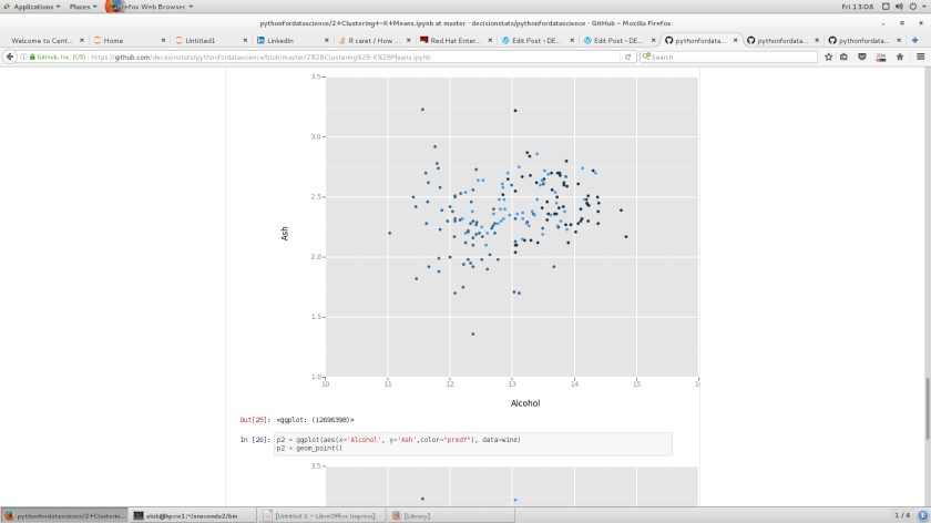
p2 = ggplot(aes(x='Alcohol', y='Ash',color="predY"), data=wine)
p2 + geom_point()

Out[26]:

<ggplot: (-9223372036842026194)>

Connecting Python with a RDBMS (Postgres)

In [1]:

import psycopg2
import pandas as pd
import sqlalchemy as sa
import time
import seaborn as sns
import re

In [2]:

!pip install psycopg2

Requirement already satisfied: psycopg2 in c:\users\dell\anaconda3\lib\site-packages

In [3]:

parameters = { 
               'username': 'postgres', 
               'password': 'root',
               'server':   'localhost',
               'database': 'datascience'
             }

In [4]:

connection= 'postgresql://{username}:{password}@{server}:5432/{database}'.format(**parameters)

In [5]:

print (connection)

postgresql://postgres:root@localhost:5432/datascience

In [6]:

engine = sa.create_engine(connection, encoding="utf-8")

In [7]:

insp = sa.inspect(engine)
db_list = insp.get_schema_names()
print(db_list)

['information_schema', 'public']

In [8]:

print(insp)

<sqlalchemy.dialects.postgresql.base.PGInspector object at 0x000000000B166748>

In [9]:

engine.table_names()

Out[9]:

['weather', 'cities', 'sales', 'sales23', 'sales77']

In [11]:

data3= pd.read_sql_query('select * from "sales77" limit 10',con=engine)

In [12]:

print(data3)

   customer_id  sales        date  product_id
0        10001    845  2017-07-05         407
1        10002   2370  2015-11-18         617
2        10003   5744  2017-02-10         928
3        10004   3230  2017-01-13         500
4        10005   8781  2017-04-23         555
5        10006   2544  2016-01-14         316
6        10007    217  2015-06-21         187
7        10008    306  2015-02-27         880
8        10009   8720  2015-09-03         900
9        10010   6137  2016-06-08         110

https://github.com/decisionstats/pythonfordatascience/blob/master/Python%2Bwith%2BPostgres%20(3).ipynb