Windows Azure and Amazon Free offer

Simple Cpu Cache Memory Organization
Image via Wikipedia

For Hi-Computing folks try out Azure for free-

http://www.microsoft.com/windowsazure/offers/popup/popup.aspx?lang=en&locale=en-US&offer=MS-AZR-0001P#compute

Windows Azure Platform
Introductory Special

This promotional offer enables you to try a limited amount of the Windows Azure platform at no charge. The subscription includes a base level of monthly compute hours, storage, data transfers, a SQL Azure database, Access Control transactions and Service Bus connections at no charge. Please note that any usage over this introductory base level will be charged at standard rates.

Included each month at no charge:

  • Windows Azure
    • 25 hours of a small compute instance
    • 500 MB of storage
    • 10,000 storage transactions
  • SQL Azure
    • 1GB Web Edition database (available for first 3 months only)
  • Windows Azure platform AppFabric
    • 100,000 Access Control transactions
    • 2 Service Bus connections
  • Data Transfers (per region)
    • 500 MB in
    • 500 MB out

Any monthly usage in excess of the above amounts will be charged at the standard rates. This introductory special will end on March 31, 2011 and all usage will then be charged at the standard rates.

Standard Rates:

Windows Azure

  • Compute*
    • Extra small instance**: $0.05 per hour
    • Small instance (default): $0.12 per hour
    • Medium instance: $0.24 per hour
    • Large instance: $0.48 per hour
    • Extra large instance: $0.96 per hour


http://aws.amazon.com/ec2/pricing/

Free Tier*

As part of AWS’s Free Usage Tier, new AWS customers can get started with Amazon EC2 for free. Upon sign-up, new AWScustomers receive the following EC2 services each month for one year:

  • 750 hours of EC2 running Linux/Unix Micro instance usage
  • 750 hours of Elastic Load Balancing plus 15 GB data processing
  • 10 GB of Amazon Elastic Block Storage (EBS) plus 1 million IOs, 1 GB snapshot storage, 10,000 snapshot Get Requests and 1,000 snapshot Put Requests
  • 15 GB of bandwidth in and 15 GB of bandwidth out aggregated across all AWS services


Paid Instances-


Standard On-Demand Instances Linux/UNIX Usage Windows Usage
Small (Default) $0.085 per hour $0.12 per hour
Large $0.34 per hour $0.48 per hour
Extra Large $0.68 per hour $0.96 per hour
Micro On-Demand Instances
Micro $0.02 per hour $0.03 per hour
High-Memory On-Demand Instances
Extra Large $0.50 per hour $0.62 per hour
Double Extra Large $1.00 per hour $1.24 per hour
Quadruple Extra Large $2.00 per hour $2.48 per hour
High-CPU On-Demand Instances
Medium $0.17 per hour $0.29 per hour
Extra Large $0.68 per hour $1.16 per hour
Cluster Compute Instances
Quadruple Extra Large $1.60 per hour N/A*
Cluster GPU Instances
Quadruple Extra Large $2.10 per hour N/A*
* Windows is not currently available for Cluster Compute or Cluster GPU Instances.


NOTE- Amazon Instance definitions differ slightly from Azure definitions

http://aws.amazon.com/ec2/instance-types/

Available Instance Types

Standard Instances

Instances of this family are well suited for most applications.

Small Instance – default*

1.7 GB memory
1 EC2 Compute Unit (1 virtual core with 1 EC2 Compute Unit)
160 GB instance storage
32-bit platform
I/O Performance: Moderate
API name: m1.small

Large Instance

7.5 GB memory
4 EC2 Compute Units (2 virtual cores with 2 EC2 Compute Units each)
850 GB instance storage
64-bit platform
I/O Performance: High
API name: m1.large

Extra Large Instance

15 GB memory
8 EC2 Compute Units (4 virtual cores with 2 EC2 Compute Units each)
1,690 GB instance storage
64-bit platform
I/O Performance: High
API name: m1.xlarge

Micro Instances

Instances of this family provide a small amount of consistent CPU resources and allow you to burst CPU capacity when additional cycles are available. They are well suited for lower throughput applications and web sites that consume significant compute cycles periodically.

Micro Instance

613 MB memory
Up to 2 EC2 Compute Units (for short periodic bursts)
EBS storage only
32-bit or 64-bit platform
I/O Performance: Low
API name: t1.micro

High-Memory Instances

Instances of this family offer large memory sizes for high throughput applications, including database and memory caching applications.

High-Memory Extra Large Instance

17.1 GB of memory
6.5 EC2 Compute Units (2 virtual cores with 3.25 EC2 Compute Units each)
420 GB of instance storage
64-bit platform
I/O Performance: Moderate
API name: m2.xlarge

High-Memory Double Extra Large Instance

34.2 GB of memory
13 EC2 Compute Units (4 virtual cores with 3.25 EC2 Compute Units each)
850 GB of instance storage
64-bit platform
I/O Performance: High
API name: m2.2xlarge

High-Memory Quadruple Extra Large Instance

68.4 GB of memory
26 EC2 Compute Units (8 virtual cores with 3.25 EC2 Compute Units each)
1690 GB of instance storage
64-bit platform
I/O Performance: High
API name: m2.4xlarge

High-CPU Instances

Instances of this family have proportionally more CPU resources than memory (RAM) and are well suited for compute-intensive applications.

High-CPU Medium Instance

1.7 GB of memory
5 EC2 Compute Units (2 virtual cores with 2.5 EC2 Compute Units each)
350 GB of instance storage
32-bit platform
I/O Performance: Moderate
API name: c1.medium

High-CPU Extra Large Instance

7 GB of memory
20 EC2 Compute Units (8 virtual cores with 2.5 EC2 Compute Units each)
1690 GB of instance storage
64-bit platform
I/O Performance: High
API name: c1.xlarge

Cluster Compute Instances

Instances of this family provide proportionally high CPU resources with increased network performance and are well suited for High Performance Compute (HPC) applications and other demanding network-bound applications. Learn more about use of this instance type for HPC applications.

Cluster Compute Quadruple Extra Large Instance

23 GB of memory
33.5 EC2 Compute Units (2 x Intel Xeon X5570, quad-core “Nehalem” architecture)
1690 GB of instance storage
64-bit platform
I/O Performance: Very High (10 Gigabit Ethernet)
API name: cc1.4xlarge

Cluster GPU Instances

Instances of this family provide general-purpose graphics processing units (GPUs) with proportionally high CPU and increased network performance for applications benefitting from highly parallelized processing, including HPC, rendering and media processing applications. While Cluster Compute Instances provide the ability to create clusters of instances connected by a low latency, high throughput network, Cluster GPU Instances provide an additional option for applications that can benefit from the efficiency gains of the parallel computing power of GPUs over what can be achieved with traditional processors. Learn moreabout use of this instance type for HPC applications.

Cluster GPU Quadruple Extra Large Instance

22 GB of memory
33.5 EC2 Compute Units (2 x Intel Xeon X5570, quad-core “Nehalem” architecture)
2 x NVIDIA Tesla “Fermi” M2050 GPUs
1690 GB of instance storage
64-bit platform
I/O Performance: Very High (10 Gigabit Ethernet)
API name: cg1.4xlarge

versus-

Windows Azure compute instances come in five unique sizes to enable complex applications and workloads.

Compute Instance Size CPU Memory Instance Storage I/O Performance
Extra Small 1 GHz 768 MB 20 GB* Low
Small 1.6 GHz 1.75 GB 225 GB Moderate
Medium 2 x 1.6 GHz 3.5 GB 490 GB High
Large 4 x 1.6 GHz 7 GB 1,000 GB High
Extra large 8 x 1.6 GHz 14 GB 2,040 GB High

*There is a limitation on the Virtual Hard Drive (VHD) size if you are deploying a Virtual Machine role on an extra small instance. The VHD can only be up to 15 GB.


Handling time and date in R

John Harrison's famous chronometer
Image via Wikipedia

One of the most frustrating things I had to do while working as financial business analysts was working with Data Time Formats in Base SAS. The syntax was simple enough and SAS was quite good with handing queries to the Oracle data base that the client was using, but remembering the different types of formats in SAS language was a challenge (there was a date9. and date6 and mmddyy etc )

Data and Time variables are particularly important variables in financial industry as almost everything is derived variable from the time (which varies) while other inputs are mostly constants. This includes interest as well as late fees and finance fees.

In R, date and time are handled quite simply-

Use the strptime( dataset, format) function to convert the character into string

For example if the variable dob is “01/04/1977) then following will convert into a date object

z=strptime(dob,”%d/%m/%Y”)

and if the same date is 01Apr1977

z=strptime(dob,"%d%b%Y")


does the same

For troubleshooting help with date and time, remember to enclose the formats

%d,%b,%m and % Y in the same exact order as the original string- and if there are any delimiters like ” -” or “/” then these delimiters are entered in exactly the same order in the format statement of the strptime

Sys.time() gives you the current date-time while the function difftime(time1,time2) gives you the time intervals( say if you have two columns as date-time variables)


What are the various formats for inputs in date time?

%a
Abbreviated weekday name in the current locale. (Also matches full name on input.)
%A
Full weekday name in the current locale. (Also matches abbreviated name on input.)
%b
Abbreviated month name in the current locale. (Also matches full name on input.)
%B
Full month name in the current locale. (Also matches abbreviated name on input.)
%c
Date and time. Locale-specific on output, "%a %b %e %H:%M:%S %Y" on input.
%d
Day of the month as decimal number (01–31).
%H
Hours as decimal number (00–23).
%I
Hours as decimal number (01–12).
%j
Day of year as decimal number (001–366).
%m
Month as decimal number (01–12).
%M
Minute as decimal number (00–59).
%p
AM/PM indicator in the locale. Used in conjunction with %I and not with %H. An empty string in some locales.
%S
Second as decimal number (00–61), allowing for up to two leap-seconds (but POSIX-compliant implementations will ignore leap seconds).
%U
Week of the year as decimal number (00–53) using Sunday as the first day 1 of the week (and typically with the first Sunday of the year as day 1 of week 1). The US convention.
%w
Weekday as decimal number (0–6, Sunday is 0).
%W
Week of the year as decimal number (00–53) using Monday as the first day of week (and typically with the first Monday of the year as day 1 of week 1). The UK convention.
%x
Date. Locale-specific on output, "%y/%m/%d" on input.
%X
Time. Locale-specific on output, "%H:%M:%S" on input.
%y
Year without century (00–99). Values 00 to 68 are prefixed by 20 and 69 to 99 by 19 – that is the behaviour specified by the 2004 POSIX standard, but it does also say ‘it is expected that in a future version the default century inferred from a 2-digit year will change’.
%Y
Year with century.
%z
Signed offset in hours and minutes from UTC, so -0800 is 8 hours behind UTC.
%Z
(output only.) Time zone as a character string (empty if not available).

Also to read the helpful documentation (especially for time zone level, and leap year seconds and differences)
http://stat.ethz.ch/R-manual/R-patched/library/base/html/difftime.html
http://stat.ethz.ch/R-manual/R-patched/library/base/html/strptime.html
http://stat.ethz.ch/R-manual/R-patched/library/base/html/Ops.Date.html
http://stat.ethz.ch/R-manual/R-patched/library/base/html/Dates.html


How to Analyze Wikileaks Data – R SPARQL

Logo for R
Image via Wikipedia

Drew Conway- one of the very very few Project R voices I used to respect until recently. declared on his blog http://www.drewconway.com/zia/

Why I Will Not Analyze The New WikiLeaks Data

and followed it up with how HE analyzed the post announcing the non-analysis.

“If you have not visited the site in a week or so you will have missed my previous post on analyzing WikiLeaks data, which from the traffic and 35 Comments and 255 Reactions was at least somewhat controversial. Given this rare spotlight I thought it would be fun to use the infochimps API to map out the geo-location of everyone that visited the blog post over the last few days. Unfortunately, after nearly two years with the same web hosting service, only today did I realize that I was not capturing daily log files for my domain”

Anyways – non American users of R Project can analyze the Wikileaks data using the R SPARQL package I would advise American friends not to use this approach or attempt to analyze any data because technically the data is still classified and it’s possession is illegal (which is the reason Federal employees and organizations receiving federal funds have advised not to use this or any WikiLeaks dataset)

https://code.google.com/p/r-sparql/

Overview

R is a programming language designed for statistics.

R Sparql allows you to run SPARQL Queries inside R and store it as a R data frame.

The main objective is to allow the integration of Ontologies with Statistics.

It requires Java and rJava installed.

Example (in R console):

> library(sparql)> data <- query("SPARQL query>","RDF file or remote SPARQL Endpoint")

and the data in a remote SPARQL  http://www.ckan.net/package/cablegate

SPARQL is an easy language to pick  up, but dammit I am not supposed to blog on my vacations.

http://code.google.com/p/r-sparql/wiki/GettingStarted

Getting Started

1. Installation

1.1 Make sure Java is installed and is the default JVM:

$ sudo apt-get install sun-java6-bin sun-java6-jre sun-java6-jdk$ sudo update-java-alternatives -s java-6-sun

1.2 Configure R to use the correct version of Java

$ sudo R CMD javareconf

1.3 Install the rJava library

$ R> install.packages("rJava")> q()

1.4 Download and install the sparql library

Download: http://code.google.com/p/r-sparql/downloads/list

$ R CMD INSTALL sparql-0.1-X.tar.gz

2. Executing a SPARQL query

2.1 Start R

#Load the librarylibrary(sparql)#Run the queryresult <- query("SELECT ... ", "http://...")#Print the resultprint(result)

3. Examples

3.1 The Query can be a string or a local file:

query("SELECT ?date ?number ?season WHERE {  ... }", "local-file.rdf")
query("my-query.rq", "local-file.rdf")

The package will detect if my-query.rq exists and will load it from the file.

3.3 The uri can be a file or an url (for remote queries):

query("SELECT ... ","local-file.db")
query("SELECT ... ","http://dbpedia.org/sparql")

3.4 Get some examples here: http://code.google.com/p/r-sparql/downloads/list

SPARQL Tutorial-

http://openjena.org/ARQ/Tutorial/index.html

Also read-

http://webr3.org/blog/linked-data/virtuoso-6-sparqlgeo-and-linked-data/

and from the favorite blog of Project R- Also known as NY Times

http://bits.blogs.nytimes.com/2010/11/15/sorting-through-the-government-data-explosion/?twt=nytimesbits

In May 2009, the Obama administration started putting raw 
government data on the Web. 
It started with 47 data sets. Today, there are more than
 270,000 government data sets, spanning every imaginable 
category from public health to foreign aid.

AsterData partners with Tableau

This chart represents several constituent comp...
Image via Wikipedia

Tableau which has been making waves recntly with its great new data visualization tool announced a partner with my old friends at AsterData. Its really cool piece of data vis and very very fast on the desktop- so I can imagine what speed it can help with AsterData’s MPP Row and Column Zingbang AND Parallel Analytical Functions

Tableau and AsterData also share the common Stanfordian connection (but it seems software is divided quite equally between Stanford, Hardvard Dropouts and North Carolina )

It remains to be seen in this announcement how much each company  can leverage the partnership or whether it turns like the SAS Institute- AsterData partnership last year or whether it is just to announce connectors in their software to talk to each other.

See a Tableau vis at

http://public.tableausoftware.com/views/geographyofdiabetes/Dashboard2?:embed=yes&:toolbar=yes

AsterData remains the guys with the potential but I would be wrong to say MapReduceSQL is as hot in December 2010 as it was in June 2009- and the elephant in the room would be Hadoop. That and Google’s continued shyness from encashing its principal comptency of handling Big Data (but hush – I signed a NDA with the Google Prediction API– so things maaaay change very rapidly on ahem that cloud)

Disclaimer- AsterData was my internship sponsor during my winter training while at Univ of  Tenn.


Data Visualization using Tableau

Image representing Tableau Software as depicte...
Image via CrunchBase

Here is a great piece of software for data visualization– the public version is free.

And you can use it for Desktop Analytics as well as BI /server versions at very low cost.

About Tableau Software

http://www.tableausoftware.com/press_release/tableau-massive-growth-hiring-q3-2010

Tableau was named by Software Magazine as the fastest growing software company in the $10 million to $30 million range in the world, and the second fastest growing software company worldwide overall. The ranking stems from the publication’s 28th annual Software 500 ranking of the world’s largest software service providers.

“We’re growing fast because the market is starving for easy-to-use products that deliver rapid-fire business intelligence to everyone. Our customers want ways to unlock their databases and produce engaging reports and dashboards,” said Christian Chabot CEO and co-founder of Tableau.

http://www.tableausoftware.com/about/who-we-are

History in the Making

Put together an Academy-Award winning professor from the nation’s most prestigious university, a savvy business leader with a passion for data, and a brilliant computer scientist. Add in one of the most challenging problems in software – making databases and spreadsheets understandable to ordinary people. You have just recreated the fundamental ingredients for Tableau.

The catalyst? A Department of Defense (DOD) project aimed at increasing people’s ability to analyze information and brought to famed Stanford professor, Pat Hanrahan. A founding member of Pixar and later its chief architect for RenderMan, Pat invented the technology that changed the world of animated film. If you know Buzz and Woody of “Toy Story”, you have Pat to thank.

Under Pat’s leadership, a team of Stanford Ph.D.s got together just down the hall from the Google folks. Pat and Chris Stolte, the brilliant computer scientist, realized that data visualization could produce large gains in people’s ability to understand information. Rather than analyzing data in text form and then creating visualizations of those findings, Pat and Chris invented a technology called VizQL™ by which visualization is part of the journey and not just the destination. Fast analytics and visualization for everyone was born.

While satisfying the DOD project, Pat and Chris met Christian Chabot, a former data analyst who turned into Jello when he saw what had been invented. The three formed a company and spun out of Stanford like so many before them (Yahoo, Google, VMWare, SUN). With Christian on board as CEO, Tableau rapidly hit one success after another: its first customer (now Tableau’s VP, Operations, Tom Walker), an OEM deal with Hyperion (now Oracle), funding from New Enterprise Associates, a PC Magazine award for “Product of the Year” just one year after launch, and now over 50,000 people in 50+ countries benefiting from the breakthrough.

also see http://www.tableausoftware.com/about/leadership

http://www.tableausoftware.com/about/board

—————————————————————————-

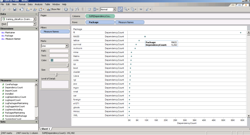
and now  a demo I ran on the Kaggle contest data (it is a csv dataset with 95000 rows)

I found Tableau works extremely good at pivoting data and visualizing it -almost like Excel on  Steroids. Download the free version here ( I dont know about an academic program (see links below) but software is not expensive at all)

http://buy.tableausoftware.com/

Desktop Personal Edition

The Personal Edition is a visual analysis and reporting solution for data stored in Excel, MS Access or Text Files. Available via download.

Product Information

$999*

Desktop Professional Edition

The Professional Edition is a visual analysis and reporting solution for data stored in MS SQL Server, MS Analysis Services, Oracle, IBM DB2, Netezza, Hyperion Essbase, Teradata, Vertica, MySQL, PostgreSQL, Firebird, Excel, MS Access or Text Files. Available via download.

Product Information

$1800*

Tableau Server

Tableau Server enables users of Tableau Desktop Professional to publish workbooks and visualizations to a server where users with web browsers can access and interact with the results. Available via download.

Product Information

Contact Us

* Price is per Named User and includes one year of maintenance (upgrades and support). Products are made available as a download immediately after purchase. You may revisit the download site at any time during your current maintenance period to access the latest releases.


Using Reshape2 for transposing datasets in R

Note Problem Statement-This is quite similar to using Proc Transpose using values in SAS. see http://analytics.ncsu.edu/sesug/2005/TU12_05.PDF
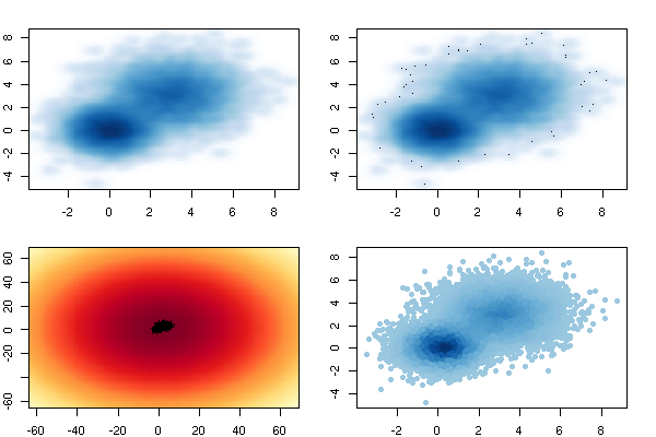
Diagram using geneplotter from R Graph Gallery
In R however this can be done as follow.
convert dataframe
Subject     Item      Score
1 Subject 1     Item 1     1
2 Subject 1     Item 2     0
3 Subject 1     Item 3     1
4 Subject 2     Item 1     1
5 Subject 2     Item 2     1
6 Subject 2      Item 3     0
to
Subject     Item 1 Item 2 Item 3 Item 4
1 Subject 1      1              0               1                 1
5 Subject 2      1              1                0                0
Note- I am using http://www.inside-r.org/pretty-r/tool for auto-generating the color coded R Code.
library("reshape2")
tDat.m<- melt(tDat)tDatCast<- acast(tDat.m,Subject~Item)
and that's it!
Another way (this one is  not recommended as it seems to take longer
 and more memory)
df.wide <- reshape(df, idvar="Subject", timevar="Item", direction="wide")