Using Google Analytics API with R:dimensions and metrics

I modified the query I wrote earlier  at http://www.decisionstats.com/using-google-analytics-with-r/to get multiple dimensions and metrics from the Google Analytics API, like hour of day,day of week to get cyclical parameters.We are adding the dimensions, and metrics to bring more depth in our analysis.Basically we are trying to do a time series analysis for forecasting web analytics data( which is basically time -stamped and rich in details ).

Basically I am modifying the dimensions and metrics parameters of the query code using the list at

http://code.google.com/apis/analytics/docs/gdata/dimsmets/dimsmets.html


query <- QueryBuilder()
query$Init(start.date = "2011-08-20",
                   end.date = "2012-08-25",
                   dimensions = c("ga:date","ga:hour","ga:dayOfWeek"),
                   metrics = c("ga:visitors","ga:visits","ga:pageviews","ga:timeOnSite"),
                   sort = c("ga:date","ga:hour","ga:dayOfWeek"),
                   table.id = paste(profiles$profile[3,3]))

#5. Make a request to get the data from the API 

ga.data <- ga$GetReportData(query)

#6. Look at the returned data 

str(ga.data)

head(ga.data$data) 

and we need the lubridate package to create a ymd:hour (time stamp)    since GA gives data aggregated at a hourly level at most. Also we need to smoothen the effect of weekend on web analytics data.

#Using package lubridate to convert character dates into time

library(lubridate)
ga.data$data[,1]=ymd(ga.data$data[,1])
ls()
dataset1=ga.data$data
names(dataset1) <- make.names(names(dataset1))
str(dataset1)
head(dataset1)

To be continued-

Using Google Analytics with R

Some code to read in data from Google Analytics data. Some modifications include adding the SSL authentication code and modifying (in bold) the table.id parameter to choose correct website from a GA profile with many websites

The Google Analytics Package files can be downloaded from http://code.google.com/p/r-google-analytics/downloads/list

It provides access to Google Analytics data natively from the R Statistical Computing programming language. You can use this library to retrieve an R data.frame with Google Analytics data. Then perform advanced statistical analysis, like time series analysis and regressions.

Supported Features

  • Access to v2 of the Google Analytics Data Export API Data Feed
  • A QueryBuilder class to simplify creating API queries
  • API response is converted directly into R as a data.frame
  • Library returns the aggregates, and confidence intervals of the metrics, dynamically if they exist
  • Auto-pagination to return more than 10,000 rows of information by combining multiple data requests. (Upper Limit 1M rows)
  • Authorization through the ClientLogin routine
  • Access to all the profiles ids for the authorized user
  • Full documentation and unit tests
Code-

> library(XML)

>

> library(RCurl)

Loading required package: bitops

>

> #Change path name in the following to the folder you downloaded the Google Analytics Package

>

> source(“C:/Users/KUs/Desktop/CANADA/R/RGoogleAnalytics/R/RGoogleAnalytics.R”)

>

> source(“C:/Users/KUs/Desktop/CANADA/R/RGoogleAnalytics/R/QueryBuilder.R”)

> # download the file needed for authentication

> download.file(url=”http://curl.haxx.se/ca/cacert.pem&#8221;, destfile=”cacert.pem”)

trying URL ‘http://curl.haxx.se/ca/cacert.pem&#8217; Content type ‘text/plain’ length 215993 bytes (210 Kb) opened

URL downloaded 210 Kb

>

> # set the curl options

> curl <- getCurlHandle()

> options(RCurlOptions = list(capath = system.file(“CurlSSL”, “cacert.pem”,

+ package = “RCurl”),

+ ssl.verifypeer = FALSE))

> curlSetOpt(.opts = list(proxy = ‘proxyserver:port’), curl = curl)

An object of class “CURLHandle” Slot “ref”: <pointer: 0000000006AA2B70>

>

> # 1. Create a new Google Analytics API object

>

> ga <- RGoogleAnalytics()

>

> # 2. Authorize the object with your Google Analytics Account Credentials

>

> ga$SetCredentials(“USERNAME”, “PASSWORD”)

>

> # 3. Get the list of different profiles, to help build the query

>

> profiles <- ga$GetProfileData()

>

> profiles #Error Check to See if we get the right website

$profile AccountName ProfileName TableId

1 dudeofdata.com dudeofdata.com ga:44926237

2 knol.google.com knol.google.com ga:45564890

3 decisionstats.com decisionstats.com ga:46751946

$total.results

total.results

1 3

>

> # 4. Build the Data Export API query

>

> #Modify the start.date and end.date parameters based on data requirements

>

> #Modify the table.id at table.id = paste(profiles$profile[X,3]) to get the X th website in your profile

> # 4. Build the Data Export API query

> query <- QueryBuilder() > query$Init(start.date = “2012-01-09”, + end.date = “2012-03-20”, + dimensions = “ga:date”,

+ metrics = “ga:visitors”,

+ sort = “ga:date”,

+ table.id = paste(profiles$profile[3,3]))

>

>

> #5. Make a request to get the data from the API

>

> ga.data <- ga$GetReportData(query)

[1] “Executing query: https://www.google.com/analytics/feeds/data?start-date=2012%2D01%2D09&end-date=2012%2D03%2D20&dimensions=ga%3Adate&metrics=ga%3Avisitors&sort=ga%3Adate&ids=ga%3A46751946&#8221;

>

> #6. Look at the returned data

>

> str(ga.data)

List of 3

$ data :’data.frame’: 72 obs. of 2 variables: ..

$ ga:date : chr [1:72] “20120109” “20120110” “20120111” “20120112” … ..

$ ga:visitors: num [1:72] 394 405 381 390 323 47 169 67 94 89 …

$ aggr.totals :’data.frame’: 1 obs. of 1 variable: ..

$ aggregate.totals: num 28348

$ total.results: num 72

>

> head(ga.data$data)

ga:date ga:visitors

1 20120109 394

2 20120110 405

3 20120111 381

4 20120112 390

5 20120113 323

6 20120114 47 >

> #Plotting the Traffic >

> plot(ga.data$data[,2],type=”l”)

Update- Some errors come from pasting Latex directly to WordPress. Here is some code , made pretty-r in case you want to play with the GA api

library(XML)

library(RCurl)

#Change path name in the following to the folder you downloaded the Google Analytics Package 

source("C:/Users/KUs/Desktop/CANADA/R/RGoogleAnalytics/R/RGoogleAnalytics.R")

source("C:/Users/KUs/Desktop/CANADA/R/RGoogleAnalytics/R/QueryBuilder.R")
# download the file needed for authentication
download.file(url="http://curl.haxx.se/ca/cacert.pem", destfile="cacert.pem")

# set the curl options
curl <- getCurlHandle()
options(RCurlOptions = list(capath = system.file("CurlSSL", "cacert.pem",
package = "RCurl"),
ssl.verifypeer = FALSE))
curlSetOpt(.opts = list(proxy = 'proxyserver:port'), curl = curl)

# 1. Create a new Google Analytics API object 

ga <- RGoogleAnalytics()

# 2. Authorize the object with your Google Analytics Account Credentials 

ga$SetCredentials("ohri2007@gmail.com", "XXXXXXX")

# 3. Get the list of different profiles, to help build the query

profiles <- ga$GetProfileData()

profiles #Error Check to See if we get the right website

# 4. Build the Data Export API query 

#Modify the start.date and end.date parameters based on data requirements 

#Modify the table.id at table.id = paste(profiles$profile[X,3]) to get the X th website in your profile 
# 4. Build the Data Export API query
query <- QueryBuilder()
query$Init(start.date = "2012-01-09",
                   end.date = "2012-03-20",
                   dimensions = "ga:date",
                   metrics = "ga:visitors",
                   sort = "ga:date",
                   table.id = paste(profiles$profile[3,3]))

#5. Make a request to get the data from the API 

ga.data <- ga$GetReportData(query)

#6. Look at the returned data 

str(ga.data)

head(ga.data$data)

#Plotting the Traffic 

plot(ga.data$data[,2],type="l")

Created by Pretty R at inside-R.org

Doing Time Series using a R GUI

The Xerox Star Workstation introduced the firs...
Image via Wikipedia

Until recently I had been thinking that RKWard was the only R GUI supporting Time Series Models-

however Bob Muenchen of http://www.r4stats.com/ was helpful to point out that the Epack Plugin provides time series functionality to R Commander.

Note the GUI helps explore various time series functionality.

Using Bulkfit you can fit various ARMA models to dataset and choose based on minimum AIC


> bulkfit(AirPassengers$x)
$res
ar d ma      AIC
[1,]  0 0  0 1790.368
[2,]  0 0  1 1618.863
[3,]  0 0  2 1522.122
[4,]  0 1  0 1413.909
[5,]  0 1  1 1397.258
[6,]  0 1  2 1397.093
[7,]  0 2  0 1450.596
[8,]  0 2  1 1411.368
[9,]  0 2  2 1394.373
[10,]  1 0  0 1428.179
[11,]  1 0  1 1409.748
[12,]  1 0  2 1411.050
[13,]  1 1  0 1401.853
[14,]  1 1  1 1394.683
[15,]  1 1  2 1385.497
[16,]  1 2  0 1447.028
[17,]  1 2  1 1398.929
[18,]  1 2  2 1391.910
[19,]  2 0  0 1413.639
[20,]  2 0  1 1408.249
[21,]  2 0  2 1408.343
[22,]  2 1  0 1396.588
[23,]  2 1  1 1378.338
[24,]  2 1  2 1387.409
[25,]  2 2  0 1440.078
[26,]  2 2  1 1393.882
[27,]  2 2  2 1392.659
$min
ar        d       ma      AIC
2.000    1.000    1.000 1378.338
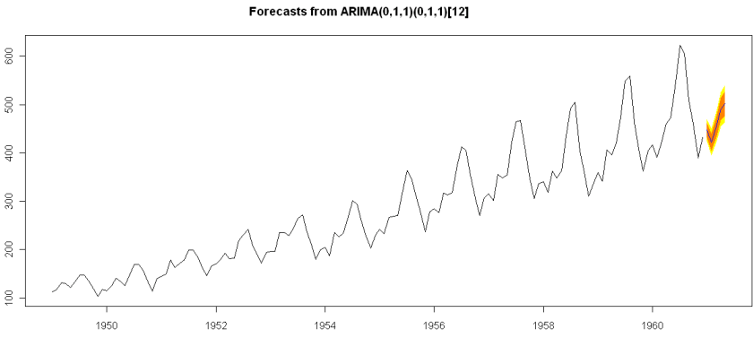
> ArimaModel.5 <- Arima(AirPassengers$x,order=c(0,1,1),
+ include.mean=1,
+   seasonal=list(order=c(0,1,1),period=12))
> ArimaModel.5
Series: AirPassengers$x
ARIMA(0,1,1)(0,1,1)[12]
Call: Arima(x = AirPassengers$x, order = c(0, 1, 1), seasonal = list(order = c(0,      1, 1), period = 12), include.mean = 1)
Coefficients:
ma1     sma1
-0.3087  -0.1074
s.e.   0.0890   0.0828
sigma^2 estimated as 135.4:  log likelihood = -507.5
AIC = 1021   AICc = 1021.19   BIC = 1029.63
> summary(ArimaModel.5, cor=FALSE)
Series: AirPassengers$x
ARIMA(0,1,1)(0,1,1)[12]
Call: Arima(x = AirPassengers$x, order = c(0, 1, 1), seasonal = list(order = c(0,      1, 1), period = 12), include.mean = 1)
Coefficients:
ma1     sma1
-0.3087  -0.1074
s.e.   0.0890   0.0828
sigma^2 estimated as 135.4:  log likelihood = -507.5
AIC = 1021   AICc = 1021.19   BIC = 1029.63
In-sample error measures:
ME        RMSE         MAE         MPE        MAPE        MASE
0.32355285 11.09952005  8.16242469  0.04409006  2.89713514  0.31563730
Dataset79 <- predar3(ArimaModel.5,fore1=5)


And I also found an interesting Ref Sheet for Time Series functions in R-

http://cran.r-project.org/doc/contrib/Ricci-refcard-ts.pdf

and a slightly more exhaustive time series ref card

http://www.statistische-woche-nuernberg-2010.org/lehre/bachelor/datenanalyse/Refcard3.pdf

Also of interest a matter of opinion on issues in Time Series Analysis in R at

http://www.stat.pitt.edu/stoffer/tsa2/Rissues.htm

Of course , if I was the sales manager for SAS ETS I would be worried given the increasing capabilities in Time Series in R. But then again some deficiencies in R GUI for Time Series-

1) Layout is not very elegant

2) Not enough documented help (atleast for the Epack GUI- and no integrated help ACROSS packages-)

3) Graphical capabilties need more help documentation to interpret the output (especially in ACF and PACF plots)

More resources on Time Series using R.

http://people.bath.ac.uk/masgs/time%20series/TimeSeriesR2004.pdf

and http://www.statoek.wiso.uni-goettingen.de/veranstaltungen/zeitreihen/sommer03/ts_r_intro.pdf

and books

http://www.springer.com/economics/econometrics/book/978-0-387-77316-2

http://www.springer.com/statistics/statistical+theory+and+methods/book/978-0-387-75960-9

http://www.springer.com/statistics/statistical+theory+and+methods/book/978-0-387-75958-6

http://www.springer.com/statistics/statistical+theory+and+methods/book/978-0-387-75966-1

Using R for Time Series in SAS


Time series: random data plus trend, with best...
Image via Wikipedia


Here is a great paper on using Time Series in R, and it specifically allows you to use just R output in Base SAS.

SAS Code

/* three methods: */

/* 1. Call R directly – Some errors are not reported to log */

x “’C:\Program Files\R\R-2.12.0\bin\r.exe’–no-save –no-restore <“”&rsourcepath\tsdiag.r””>””&rsourcepath\tsdiag.out”””;

/* include the R log in the SAS log */7data _null_;

infile “&rsourcepath\tsdiag.out”;

file log;

input;

put ’R LOG: ’ _infile_;

run;

/* include the image in the sas output.Specify a file if you are not using autogenerated html output */

ods html;

data _null_;

file print;

put “<IMG SRC=’” “&rsourcepath\plot.png” “’ border=’0’>”;

put “<IMG SRC=’” “&rsourcepath\acf.png” “’ border=’0’>”;

put “<IMG SRC=’” “&rsourcepath\pacf.png” “’ border=’0’>”;

put “<IMG SRC=’” “&rsourcepath\spect.png” “’ border=’0’>”;

put “<IMG SRC=’” “&rsourcepath\fcst.png” “’ border=’0’>”;

run;

ods html close;

The R code to create a time series plot is quite elegant though-


library(tseries)

air <- AirPassengers #Datasetname

ts.plot(air)

acf(air)

pacf(air)

plot(decompose(air))

air.fit <- arima(air,order=c(0,1,1), seasonal=list(order=c(0,1,1), period=12) #The ARIMA Model Based on PACF and ACF Graphs

tsdiag(air.fit)

library(forecast)

air.forecast <- forecast(air.fit)

plot.forecast(air.forecast)

You can download the fascinating paper from the Analytics NCSU Website http://analytics.ncsu.edu/sesug/2008/ST-146.pdf

About the Author-

Sam Croker has a MS in Statistics from the University of South Carolina and has over ten years of experience in analytics.   His research interests are in time series analysis and forecasting with focus on stream-flow analysis.  He is currently using SAS, R and other analytical tools for fraud and abuse detection in Medicare and Medicaid data. He also has experience in analyzing, modeling and forecasting in the finance, marketing, hospitality, retail and pharmaceutical industries.

China biggest threat to Indian Software in 5 years: Indian Tech CEO

The Hall of Prayer for Good Harvest, Temple of...
Image via Wikipedia

An interview with a noted Indian Software CEO, mentions China the possible biggest threat in next 5 years at  http://www.thehindubusinessline.com/2010/10/13/stories/2010101353180700.htm


China could be the biggest threat to India in next five years, positioning itself as the lowest-cost manpower supplier in the IT sector by 2015, according to Mr Vineet Nayar, CEO, HCL Technologies.

“I believe it (China) is the biggest threat in the next five years that we are going to face…So India will have to up its game,” he told reporters on sidelines of ‘Directions’, the company’s annual town hall.

Terming China, as both “threat and opportunity”, Mr Nayar said that India will have to find alternate “differentiators” than the ones it currently has. Despite issues of language and the purported inability to scale-up, China has sharpened its technological and innovation edge, he added.

“Look at the technology companies from China…how does that fit in with the assumption that they (China) do not understand English or technology. They are producing cutting edge technology at a price which is lower than everyone else,” he said.

Manpower

By 2015, Mr Nayar said, China will be the lowest cost manpower supplier in IT sector to the world

——————————————————————————————–

I wonder how he did his forecast. Did he do a time series analysis using a software, did he peer into his crystal ball, or did he spend a lot of time brainstorming with his strategic macro economic team on Chinese threat.

China has various advantages over India (and in fact the US)-

1) Big pool of reliable scientific manpower

2) State funded education in higher studies and STEM

3) Increasing exposure with the West-English speaking is no longer an issue. Almost 50 % of Grad Students in the US in STEM and certain sectors are Chinese and they not only retain fraternal ties with the motherland- they often remain un-assimilated with American Culture mainstream. or they have a separate interaction with fellow American Chinese and seperate with American Americans.

Chinese suffer from some disadvantages in software-

1) Communism Perception- Just because the Govt is communist and likes to confront US once a year (and India twice a month)- is no excuse for the hapless Chinese startup guy to lose out on software outsourcing contracts. unfortunately there have been reported cases where sneak codes have been inserted in code deliverables for American partners, just like American companies are forced to work with DoD (especially in software, embedded chips and telecom)

If you have 10000 lines of code delivered by your Chinese partner, how sure are you of going through each line of code for each sub routine or call procedure.

2) English- Chinese accent is like Chinese cooking. Unique- many Chinese are unable to master the different style of English even after years (derived from Latin and Indo European class of languages)

Sales jobs tend to go to American trained Chinese or to Westerners.

In Indian software companies, accent is a lesser problem.

———————————————————————————-

The biggest threat to Indian software in 5 years is actually Indian software itself- Can it evolve and mature to a product based model from a service only model.

Can Indian software partner with Chinese companies and maybe teach the Indian government why friendship is more profitable than envy and suspicion. If the US and China can trade enormously despite annual tensions, why cant Indian services do the same- if they lose this opportunity, US companies will likely bypass them and create the same GE/McKinsey style backoffices that started the Indian offshoring phenomenon.

3) Lastly- what did the poor American grad student do to deserve that even if devotes years to study STEM (and being called a Geek and Nerd) his job will get outsourced to India or China (if not now- in his 30s or worse in his 40s). Talk to any middle aged IT chap in the US who is middle class- and India and China would figure in why he still worries about his overpriced mortgage.

Unless the US wants only Twitter and Facebook as dominant technologies in the 21 st century.

Amen.


%d bloggers like this: