Doing Time Series using a R GUI

The Xerox Star Workstation introduced the firs...
Image via Wikipedia

Until recently I had been thinking that RKWard was the only R GUI supporting Time Series Models-

however Bob Muenchen of http://www.r4stats.com/ was helpful to point out that the Epack Plugin provides time series functionality to R Commander.

Note the GUI helps explore various time series functionality.

Using Bulkfit you can fit various ARMA models to dataset and choose based on minimum AIC


> bulkfit(AirPassengers$x)
$res
ar d ma      AIC
[1,]  0 0  0 1790.368
[2,]  0 0  1 1618.863
[3,]  0 0  2 1522.122
[4,]  0 1  0 1413.909
[5,]  0 1  1 1397.258
[6,]  0 1  2 1397.093
[7,]  0 2  0 1450.596
[8,]  0 2  1 1411.368
[9,]  0 2  2 1394.373
[10,]  1 0  0 1428.179
[11,]  1 0  1 1409.748
[12,]  1 0  2 1411.050
[13,]  1 1  0 1401.853
[14,]  1 1  1 1394.683
[15,]  1 1  2 1385.497
[16,]  1 2  0 1447.028
[17,]  1 2  1 1398.929
[18,]  1 2  2 1391.910
[19,]  2 0  0 1413.639
[20,]  2 0  1 1408.249
[21,]  2 0  2 1408.343
[22,]  2 1  0 1396.588
[23,]  2 1  1 1378.338
[24,]  2 1  2 1387.409
[25,]  2 2  0 1440.078
[26,]  2 2  1 1393.882
[27,]  2 2  2 1392.659
$min
ar        d       ma      AIC
2.000    1.000    1.000 1378.338
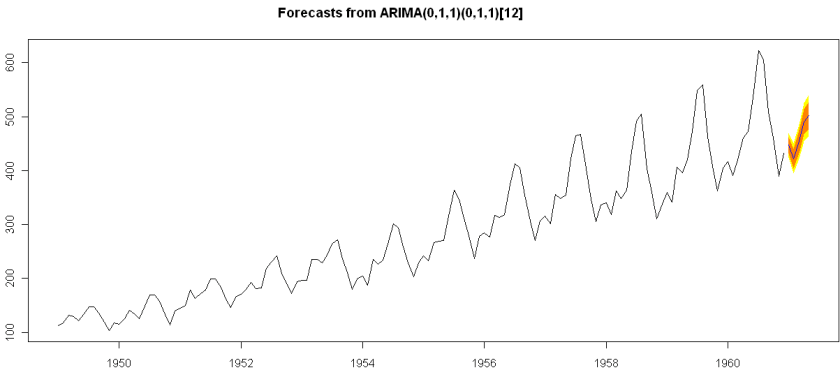
> ArimaModel.5 <- Arima(AirPassengers$x,order=c(0,1,1),
+ include.mean=1,
+   seasonal=list(order=c(0,1,1),period=12))
> ArimaModel.5
Series: AirPassengers$x
ARIMA(0,1,1)(0,1,1)[12]
Call: Arima(x = AirPassengers$x, order = c(0, 1, 1), seasonal = list(order = c(0,      1, 1), period = 12), include.mean = 1)
Coefficients:
ma1     sma1
-0.3087  -0.1074
s.e.   0.0890   0.0828
sigma^2 estimated as 135.4:  log likelihood = -507.5
AIC = 1021   AICc = 1021.19   BIC = 1029.63
> summary(ArimaModel.5, cor=FALSE)
Series: AirPassengers$x
ARIMA(0,1,1)(0,1,1)[12]
Call: Arima(x = AirPassengers$x, order = c(0, 1, 1), seasonal = list(order = c(0,      1, 1), period = 12), include.mean = 1)
Coefficients:
ma1     sma1
-0.3087  -0.1074
s.e.   0.0890   0.0828
sigma^2 estimated as 135.4:  log likelihood = -507.5
AIC = 1021   AICc = 1021.19   BIC = 1029.63
In-sample error measures:
ME        RMSE         MAE         MPE        MAPE        MASE
0.32355285 11.09952005  8.16242469  0.04409006  2.89713514  0.31563730
Dataset79 <- predar3(ArimaModel.5,fore1=5)


And I also found an interesting Ref Sheet for Time Series functions in R-

http://cran.r-project.org/doc/contrib/Ricci-refcard-ts.pdf

and a slightly more exhaustive time series ref card

http://www.statistische-woche-nuernberg-2010.org/lehre/bachelor/datenanalyse/Refcard3.pdf

Also of interest a matter of opinion on issues in Time Series Analysis in R at

http://www.stat.pitt.edu/stoffer/tsa2/Rissues.htm

Of course , if I was the sales manager for SAS ETS I would be worried given the increasing capabilities in Time Series in R. But then again some deficiencies in R GUI for Time Series-

1) Layout is not very elegant

2) Not enough documented help (atleast for the Epack GUI- and no integrated help ACROSS packages-)

3) Graphical capabilties need more help documentation to interpret the output (especially in ACF and PACF plots)

More resources on Time Series using R.

http://people.bath.ac.uk/masgs/time%20series/TimeSeriesR2004.pdf

and http://www.statoek.wiso.uni-goettingen.de/veranstaltungen/zeitreihen/sommer03/ts_r_intro.pdf

and books

http://www.springer.com/economics/econometrics/book/978-0-387-77316-2

http://www.springer.com/statistics/statistical+theory+and+methods/book/978-0-387-75960-9

http://www.springer.com/statistics/statistical+theory+and+methods/book/978-0-387-75958-6

http://www.springer.com/statistics/statistical+theory+and+methods/book/978-0-387-75966-1

Using R for Time Series in SAS


Time series: random data plus trend, with best...
Image via Wikipedia


Here is a great paper on using Time Series in R, and it specifically allows you to use just R output in Base SAS.

SAS Code

/* three methods: */

/* 1. Call R directly – Some errors are not reported to log */

x “’C:\Program Files\R\R-2.12.0\bin\r.exe’–no-save –no-restore <“”&rsourcepath\tsdiag.r””>””&rsourcepath\tsdiag.out”””;

/* include the R log in the SAS log */7data _null_;

infile “&rsourcepath\tsdiag.out”;

file log;

input;

put ’R LOG: ’ _infile_;

run;

/* include the image in the sas output.Specify a file if you are not using autogenerated html output */

ods html;

data _null_;

file print;

put “<IMG SRC=’” “&rsourcepath\plot.png” “’ border=’0’>”;

put “<IMG SRC=’” “&rsourcepath\acf.png” “’ border=’0’>”;

put “<IMG SRC=’” “&rsourcepath\pacf.png” “’ border=’0’>”;

put “<IMG SRC=’” “&rsourcepath\spect.png” “’ border=’0’>”;

put “<IMG SRC=’” “&rsourcepath\fcst.png” “’ border=’0’>”;

run;

ods html close;

The R code to create a time series plot is quite elegant though-


library(tseries)

air <- AirPassengers #Datasetname

ts.plot(air)

acf(air)

pacf(air)

plot(decompose(air))

air.fit <- arima(air,order=c(0,1,1), seasonal=list(order=c(0,1,1), period=12) #The ARIMA Model Based on PACF and ACF Graphs

tsdiag(air.fit)

library(forecast)

air.forecast <- forecast(air.fit)

plot.forecast(air.forecast)

You can download the fascinating paper from the Analytics NCSU Website http://analytics.ncsu.edu/sesug/2008/ST-146.pdf

About the Author-

Sam Croker has a MS in Statistics from the University of South Carolina and has over ten years of experience in analytics.   His research interests are in time series analysis and forecasting with focus on stream-flow analysis.  He is currently using SAS, R and other analytical tools for fraud and abuse detection in Medicare and Medicaid data. He also has experience in analyzing, modeling and forecasting in the finance, marketing, hospitality, retail and pharmaceutical industries.

%d bloggers like this: